Bem-Estar

Autor

Afiliação

Roney Fraga Souza

Universidade Federal de Mato Grosso

Por onde começar?

Material da aula: os slides são o PDF do capítulo 33 do Varian, embarcado abaixo. Use a barra de rolagem ou os controles do leitor para navegar.

Abrir o PDF em tela cheia, ou acessar na pequena janela abaixo ↓.

Material complementar: aulas em vídeo do Prof. Selçuk Özyurt (York University), playlist com 8 aulas sobre o tema.

Nota 16.1: Agregação de preferências

Desenvolvimento Teórico

Suponha uma sociedade com \(n\) indivíduos, cada um com uma preferência transitiva \(\succsim_i\) sobre um conjunto de alternativas. O problema da agregação consiste em construir uma ordenação social \(\succsim\) a partir do perfil \((\succsim_1, \ldots, \succsim_n)\) que represente coletivamente as preferências individuais.

A tentativa intuitiva é a regra da maioria 2 a 2: a sociedade prefere \(X\) a \(Y\) se a maioria dos indivíduos prefere \(X\) a \(Y\). O problema é que essa regra pode não preservar transitividade — ou seja, a ordenação social pode apresentar ciclos, ainda que cada ordenação individual seja transitiva. O exemplo clássico é o paradoxo de Condorcet.

Exemplo: o paradoxo de Condorcet

Considere 3 votantes e 3 alternativas \(X\), \(Y\), \(Z\) com o seguinte perfil:

Votante	1ª escolha	2ª escolha	3ª escolha
1	\(X\)	\(Y\)	\(Z\)
2	\(Y\)	\(Z\)	\(X\)
3	\(Z\)	\(X\)	\(Y\)

Aplicando a regra da maioria 2 a 2:

Confronto	Vota em 1º	Vota em 2º	Vota em 3º	Vencedor (maioria)
\(X\) vs \(Y\)	\(X\)	\(Y\)	\(X\)	\(X \succ Y\)
\(Y\) vs \(Z\)	\(Y\)	\(Y\)	\(Z\)	\(Y \succ Z\)
\(X\) vs \(Z\)	\(X\)	\(Z\)	\(Z\)	\(Z \succ X\)

A ordenação social resultante é \(X \succ Y \succ Z \succ X\) — um ciclo. A regra da maioria, mesmo aplicada a preferências individuais transitivas, gera uma ordenação social não transitiva.

Esse resultado motiva a busca por axiomas que uma boa regra de agregação deveria satisfazer — caminho que leva ao teorema de Arrow (Note 16.2).

Referências

Ver Varian (2012, cap. 33, §33.1).

Nota 16.2: Teorema da Impossibilidade de Arrow

Os quatro axiomas

Arrow (Arrow, 1963) propôs quatro axiomas que uma regra de agregação social \(f\) deveria satisfazer:

• (a) Domínio universal: \(f\) aceita qualquer perfil de preferências individuais transitivas e completas. Não pode haver restrição prévia sobre quais perfis são admissíveis.
• (b) Pareto fraco: se todo indivíduo prefere \(X\) a \(Y\), então a ordenação social prefere \(X\) a \(Y\).
• (c) Independência das alternativas irrelevantes (IIA): a ordenação social entre \(X\) e \(Y\) depende apenas de como cada indivíduo ordena \(X\) e \(Y\) — não depende de como qualquer outra alternativa é ordenada.
• (d) Não-ditadura: não existe um indivíduo \(i\) cujas preferências determinem a ordenação social independentemente das preferências dos demais.

Enunciado

Com pelo menos 3 alternativas e pelo menos 2 indivíduos, não existe regra de agregação social \(f\) que satisfaça simultaneamente os quatro axiomas (a)–(d).

Interpretação

O teorema de Arrow é um resultado de impossibilidade: nenhuma regra de agregação razoável existe se exigirmos os quatro axiomas em conjunto. As três saídas usuais na literatura são:

1. Restringir o domínio — abrir mão do axioma (a). Por exemplo, se todas as preferências forem unimodais (cada indivíduo tem uma alternativa preferida e a utilidade decresce nas duas direções), a regra da maioria escolhe a preferida do votante mediano (teorema do votante mediano de Black).
2. Abandonar IIA — abrir mão do axioma (c). Permite usar utilidades cardinais comparáveis entre indivíduos, abrindo espaço para funções de bem-estar social (Note 16.3).
3. Aceitar ditadura — abrir mão do axioma (d), o que politicamente raramente é aceitável.

Referências

Ver Varian (2012, cap. 33, §33.2); Arrow (1963).

Nota 16.3: Funções de Bem-Estar Social

Símbolo	Significado
\(u_A\), \(u_B\)	utilidades dos indivíduos \(A\) e \(B\)
\(W\)	função de bem-estar social (BES)
\(\alpha, \beta\)	pesos distributivos (\(\alpha, \beta > 0\))

Desenvolvimento Teórico

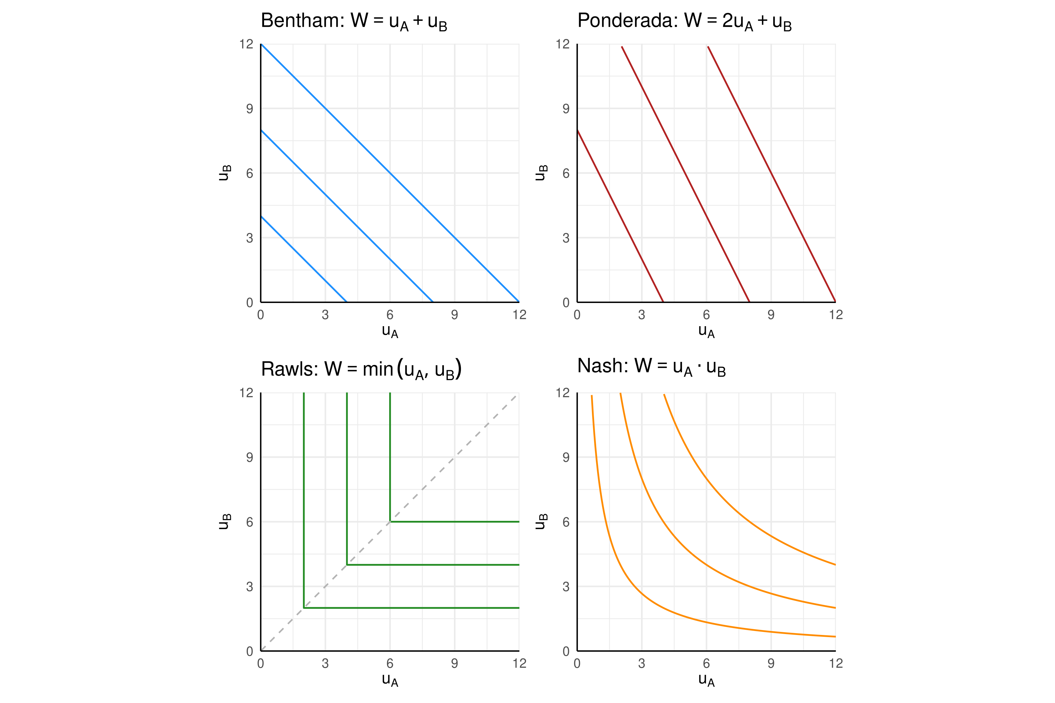
Uma função de bem-estar social (BES) atribui um número real \(W\) a cada perfil de utilidades individuais \((u_A, u_B)\). Diferentes formas funcionais incorporam diferentes juízos distributivos. As quatro mais comuns são:

1. Bentham (utilitarista): \(W = u_A + u_B\). Soma simples; só importa a soma das utilidades, não como elas se distribuem.
2. Utilitarista ponderada: \(W = \alpha\, u_A + \beta\, u_B\), com \(\alpha, \beta > 0\). Bentham é caso particular (\(\alpha = \beta\)). Pesos diferentes refletem juízos sobre quem “merece” mais.
3. Rawlsiana (maximin): \(W = \min(u_A, u_B)\). O bem-estar social é determinado pelo indivíduo em pior situação. Igualitarismo extremo.
4. Nash: \(W = u_A \cdot u_B\). Produto das utilidades; penaliza desigualdade extrema sem exigir igualdade estrita.

A classe Bergson–Samuelson generaliza todas as anteriores: qualquer função \(W = W(u_A, u_B)\) monotônica e crescente em cada argumento é uma BES de Bergson–Samuelson. Bentham, ponderada, Rawls e Nash são casos particulares dentro dessa classe.

Implementação em R

Curvas de indiferença sociais (locus de pontos \((u_A, u_B)\) com \(W\) constante) para cada forma funcional:

cor1 <- "dodgerblue"
cor2 <- "firebrick"
cor3 <- "forestgreen"
cor4 <- "darkorange"

# Bentham: u_A + u_B = W
W_b <- c(4, 8, 12)
df_bentham <- expand.grid(u_A = seq(0, 12, length.out = 100), W = W_b) |>
  mutate(u_B = W - u_A) |>
  filter(u_B >= 0, u_B <= 12)

p1 <- ggplot(df_bentham, aes(u_A, u_B, group = W)) +
  geom_line(color = cor1, linewidth = 1) +
  coord_fixed(xlim = c(0, 12), ylim = c(0, 12), expand = FALSE) +
  labs(title = TeX("Bentham: $W = u_A + u_B$"),
       x = TeX("$u_A$"), y = TeX("$u_B$")) +
  theme_minimal(base_size = 20) +
  theme(axis.line = element_line(color = "black", linewidth = 0.8))

# Ponderada: 2 u_A + u_B = W
W_p <- c(8, 16, 24)
df_pond <- expand.grid(u_A = seq(0, 12, length.out = 100), W = W_p) |>
  mutate(u_B = W - 2 * u_A) |>
  filter(u_B >= 0, u_B <= 12)

p2 <- ggplot(df_pond, aes(u_A, u_B, group = W)) +
  geom_line(color = cor2, linewidth = 1) +
  coord_fixed(xlim = c(0, 12), ylim = c(0, 12), expand = FALSE) +
  labs(title = TeX("Ponderada: $W = 2 u_A + u_B$"),
       x = TeX("$u_A$"), y = TeX("$u_B$")) +
  theme_minimal(base_size = 20) +
  theme(axis.line = element_line(color = "black", linewidth = 0.8))

# Rawls: min(u_A, u_B) = W -> "L"
W_r <- c(2, 4, 6)
df_rawls <- do.call(rbind, lapply(W_r, function(w) {
  rbind(
    data.frame(u_A = w, u_B = seq(w, 12, length.out = 50), W = w),
    data.frame(u_A = seq(w, 12, length.out = 50), u_B = w, W = w)
  )
}))

p3 <- ggplot(df_rawls, aes(u_A, u_B, group = W)) +
  geom_line(color = cor3, linewidth = 1) +
  geom_abline(slope = 1, intercept = 0, color = "gray70", linetype = "dashed") +
  coord_fixed(xlim = c(0, 12), ylim = c(0, 12), expand = FALSE) +
  labs(title = TeX("Rawls: $W = \\min(u_A, u_B)$"),
       x = TeX("$u_A$"), y = TeX("$u_B$")) +
  theme_minimal(base_size = 20) +
  theme(axis.line = element_line(color = "black", linewidth = 0.8))

# Nash: u_A * u_B = W -> hipérbole
W_n <- c(8, 24, 48)
df_nash <- expand.grid(u_A = seq(0.5, 12, length.out = 200), W = W_n) |>
  mutate(u_B = W / u_A) |>
  filter(u_B <= 12)

p4 <- ggplot(df_nash, aes(u_A, u_B, group = W)) +
  geom_line(color = cor4, linewidth = 1) +
  coord_fixed(xlim = c(0, 12), ylim = c(0, 12), expand = FALSE) +
  labs(title = TeX("Nash: $W = u_A \\cdot u_B$"),
       x = TeX("$u_A$"), y = TeX("$u_B$")) +
  theme_minimal(base_size = 20) +
  theme(axis.line = element_line(color = "black", linewidth = 0.8))

(p1 + p2) / (p3 + p4)

Cada painel mostra três níveis crescentes de bem-estar social: Bentham e ponderada produzem retas paralelas; Rawls produz cantos em “L” sobre a diagonal \(u_A = u_B\) (linha cinza); Nash produz hipérboles.

Referências

Ver Varian (2012, cap. 33, §33.3).

Nota 16.4: Maximização da BES sobre a Fronteira de Possibilidades de Utilidade

Símbolo	Significado
\(u_A\), \(u_B\)	utilidades dos indivíduos \(A\) e \(B\)
\(W\)	função de bem-estar social
UPF	Fronteira de Possibilidades de Utilidade
\(u_B = 10 - 0{,}1\, u_A^2\)	UPF côncava assumida no exercício

Desenvolvimento Teórico

A Fronteira de Possibilidades de Utilidade (UPF) é o conjunto de pares \((u_A, u_B)\) que correspondem a alocações Pareto-eficientes da economia. Pontos abaixo da UPF são tecnicamente alcançáveis mas Pareto-ineficientes; pontos acima são inviáveis.

O problema do planejador social é escolher um ponto sobre a UPF que maximize a função de bem-estar social \(W(u_A, u_B)\):

\[\max_{(u_A,\, u_B)} \; W(u_A, u_B) \quad \text{s.a.} \quad (u_A, u_B) \in \text{UPF}.\]

Diferentes formas de \(W\) (Bentham, Rawls, Nash, etc. — Note 16.3) selecionam pontos diferentes sobre a mesma UPF. O exercício a seguir ilustra isso para uma UPF côncava simples.

Exercício Resolvido

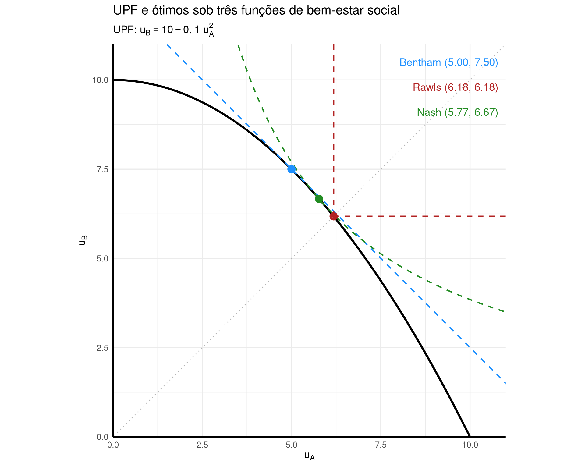
Suponha a UPF \(u_B = 10 - 0{,}1\, u_A^2\), com \(u_A \in [0, 10]\) e \(u_B \in [0, 10]\). Encontrar o ponto socialmente ótimo sob cada uma das três regras (Bentham, Rawls, Nash).

Passo 1: Bentham — maximizar \(u_A + u_B\)

Substituindo a UPF na BES:

\[\begin{aligned} W(u_A) & = u_A + (10 - 0{,}1\, u_A^2) \\[6pt] & = 10 + u_A - 0{,}1\, u_A^2 \end{aligned}\]

Condição de primeira ordem:

\[\frac{dW}{du_A} = 1 - 0{,}2\, u_A = 0 \quad \Rightarrow \quad u_A^* = 5.\]

Substituindo na UPF: \(u_B^* = 10 - 0{,}1 \cdot 25 = 7{,}5\).

Passo 2: Rawls — maximizar \(\min(u_A, u_B)\)

A solução está na diagonal \(u_A = u_B\) (acima da diagonal o gargalo é \(u_B\); abaixo é \(u_A\)). Igualando \(u_A = u_B\) na UPF:

\[\begin{aligned} u_A & = 10 - 0{,}1\, u_A^2 \\[6pt] 0{,}1\, u_A^2 + u_A - 10 & = 0 \\[6pt] u_A^2 + 10\, u_A - 100 & = 0 \quad \text{(multiplicar por 10)} \end{aligned}\]

Aplicando a fórmula de Bhaskara (descartando a raiz negativa):

\[u_A = \frac{-10 + \sqrt{100 + 400}}{2} = \frac{-10 + 10\sqrt 5}{2} = 5(\sqrt 5 - 1) \approx 6{,}18.\]

Passo 3: Nash — maximizar \(u_A \cdot u_B\)

Substituindo:

\[\begin{aligned} W(u_A) & = u_A \cdot (10 - 0{,}1\, u_A^2) \\[6pt] & = 10\, u_A - 0{,}1\, u_A^3 \end{aligned}\]

Condição de primeira ordem:

\[\frac{dW}{du_A} = 10 - 0{,}3\, u_A^2 = 0 \quad \Rightarrow \quad u_A^2 = \frac{100}{3} \quad \Rightarrow \quad u_A^* = \frac{10}{\sqrt 3} \approx 5{,}77.\]

Substituindo na UPF: \(u_B^* = 10 - 0{,}1 \cdot 100/3 = 10 - 10/3 \approx 6{,}67\).

Comparação dos três ótimos:

Regra	\(u_A^*\)	\(u_B^*\)	Valor de \(W\)	Distribuição
Bentham	\(5{,}00\)	\(7{,}50\)	\(12{,}50\)	\(A\) recebe menos
Rawls	\(6{,}18\)	\(6{,}18\)	\(6{,}18\)	igualitária
Nash	\(5{,}77\)	\(6{,}67\)	\(38{,}49\)	intermediária

Implementação em R

cor1 <- "dodgerblue"   # Bentham
cor2 <- "firebrick"    # Rawls
cor3 <- "forestgreen"  # Nash

# UPF: u_B = 10 - 0.1 u_A^2
df_upf <- data.frame(u_A = seq(0, 10, length.out = 200)) |>
  mutate(u_B = 10 - 0.1 * u_A^2)

# Pontos ótimos
ua_b <- 5
ub_b <- 7.5
ua_r <- 5 * (sqrt(5) - 1)
ub_r <- ua_r
ua_n <- 10 / sqrt(3)
ub_n <- 10 - 0.1 * ua_n^2

opts <- data.frame(
  u_A  = c(ua_b, ua_r, ua_n),
  u_B  = c(ub_b, ub_r, ub_n),
  rule = c("Bentham", "Rawls", "Nash")
)

# Curvas de indiferença social tangentes
W_b <- ua_b + ub_b               # 12.5
df_ic_b <- data.frame(u_A = seq(0, 12.5, length.out = 100)) |>
  mutate(u_B = W_b - u_A) |>
  filter(u_B >= 0, u_B <= 11)

# Rawls: "L" no ponto (ua_r, ub_r) — dois segmentos para evitar
# que geom_line conecte os endpoints e dobre o segmento vertical
df_ic_r <- rbind(
  data.frame(u_A = ua_r, u_B = seq(ua_r, 11, length.out = 50), seg = "v"),
  data.frame(u_A = seq(ua_r, 11, length.out = 50), u_B = ua_r, seg = "h")
)

# Nash: u_A * u_B = W_n
W_n <- ua_n * ub_n
df_ic_n <- data.frame(u_A = seq(0.5, 11, length.out = 200)) |>
  mutate(u_B = W_n / u_A) |>
  filter(u_B <= 11)

ggplot() +
  geom_line(data = df_upf,  aes(u_A, u_B), color = "black", linewidth = 1.2) +
  geom_line(data = df_ic_b, aes(u_A, u_B), color = cor1, linewidth = 0.8, linetype = "dashed") +
  geom_line(data = df_ic_r, aes(u_A, u_B, group = seg), color = cor2, linewidth = 0.8, linetype = "dashed") +
  geom_line(data = df_ic_n, aes(u_A, u_B), color = cor3, linewidth = 0.8, linetype = "dashed") +
  geom_point(data = opts[opts$rule == "Bentham", ], aes(u_A, u_B), color = cor1, size = 4) +
  geom_point(data = opts[opts$rule == "Rawls", ],   aes(u_A, u_B), color = cor2, size = 4) +
  geom_point(data = opts[opts$rule == "Nash", ],    aes(u_A, u_B), color = cor3, size = 4) +
  annotate("text", x = 10.8, y = 10.5,
           label = sprintf("Bentham (%.2f, %.2f)", ua_b, ub_b),
           color = cor1, hjust = 1) +
  annotate("text", x = 10.8, y = 9.8,
           label = sprintf("Rawls (%.2f, %.2f)", ua_r, ub_r),
           color = cor2, hjust = 1) +
  annotate("text", x = 10.8, y = 9.1,
           label = sprintf("Nash (%.2f, %.2f)", ua_n, ub_n),
           color = cor3, hjust = 1) +
  geom_abline(slope = 1, intercept = 0, color = "gray70", linetype = "dotted") +
  coord_fixed(xlim = c(0, 11), ylim = c(0, 11), expand = FALSE) +
  labs(title = "UPF e ótimos sob três funções de bem-estar social",
       subtitle = TeX("UPF: $u_B = 10 - 0{,}1\\, u_A^2$"),
       x = TeX("$u_A$"), y = TeX("$u_B$")) +
  theme_minimal(base_size = 13) +
  theme(axis.line = element_line(color = "black", linewidth = 0.8))

A UPF é a curva preta côncava. Cada ponto colorido é o ótimo sob uma regra de BES, e a curva pontilhada da mesma cor é a curva de indiferença social tangente à UPF naquele ponto.

Interpretação

Cada regra incorpora um juízo distributivo distinto:

• Bentham é insensível à distribuição: maximiza a soma das utilidades. Como a UPF é mais “produtiva” para valores baixos de \(u_A\) (a inclinação \(-0{,}2 u_A\) fica menos íngreme perto de \(u_A = 0\)), o ótimo de Bentham fica fora da diagonal — \(A\) recebe menos do que \(B\).
• Rawls é igualitarista extremo: força o ponto à diagonal \(u_A = u_B\). Ignora ganhos de soma se eles vierem com desigualdade.
• Nash é intermediário: penaliza desigualdade extrema (multiplicar por zero zera o produto), mas não exige igualdade estrita.

Os três pontos sobre a mesma UPF ilustram que a escolha de regra de BES é uma escolha de juízo de valor sobre distribuição — não um problema técnico.

Conexão com o 2º Teorema do Bem-Estar: qualquer ponto da UPF é alcançável como equilíbrio competitivo após uma redistribuição lump-sum das dotações iniciais. Ou seja, o planejador pode usar mercados competitivos para implementar o ótimo escolhido, desde que possa redistribuir riqueza inicial sem distorcer preços. Ver o capítulo de equilíbrio geral para a formalização do equilíbrio competitivo (em particular Note 14.7).

Referências

Ver Varian (2012, cap. 33, §33.4).

Nota 16.5: Alocações justas e livres de inveja (envy-free)

Desenvolvimento Teórico

Uma alocação \(\{x_i\}\) entre indivíduos é:

• Livre de inveja (ou envy-free) se nenhum indivíduo prefere a cesta de outro à própria, isto é, \(u_i(x_i) \geq u_i(x_j)\) para todo par \(i, j\).
• Justa (fair, no sentido de Foley–Varian) se for Pareto-eficiente e livre de inveja.

A noção de equidade aqui é puramente ordinal — não exige comparação interpessoal de utilidades. Cada indivíduo julga apenas com sua própria função de utilidade.

Resultado clássico (Varian, 1974): numa economia de troca, partindo da divisão igual da dotação agregada e permitindo trocas em equilíbrio competitivo, o equilíbrio resultante é uma alocação justa. Intuição: a divisão igual é livre de inveja por construção (todos têm a mesma cesta inicial); o equilíbrio competitivo é Pareto-eficiente (1º Teorema do Bem-Estar); e como ambos os indivíduos enfrentam os mesmos preços, nenhum poderia ter comprado a cesta do outro com sua riqueza — logo, a propriedade de não-inveja é preservada.

Exemplo numérico

Considere uma economia com 2 indivíduos \(A\) e \(B\) e 2 bens \(x\) e \(y\). Dotação agregada = \((10, 10)\), dividida igualmente: \(\omega_A = \omega_B = (5, 5)\). Utilidades:

\[u_A(x, y) = x^{0{,}7}\, y^{0{,}3}, \qquad u_B(x, y) = x^{0{,}3}\, y^{0{,}7}.\]

Note a assimetria: \(A\) valoriza mais \(x\) e \(B\) valoriza mais \(y\). Após trocas, suponha que se chegue à alocação \((x_A, y_A) = (7, 3)\) e \((x_B, y_B) = (3, 7)\) (factibilidade: \(7 + 3 = 10\) em cada bem). Verificar se é livre de inveja:

Comparação	Cálculo	Valor
\(A\) na própria cesta: \(u_A(7, 3)\)	\(7^{0{,}7} \cdot 3^{0{,}3}\)	\(\approx 5{,}43\)
\(A\) na cesta de \(B\): \(u_A(3, 7)\)	\(3^{0{,}7} \cdot 7^{0{,}3}\)	\(\approx 3{,}87\)
\(B\) na própria cesta: \(u_B(3, 7)\)	\(3^{0{,}3} \cdot 7^{0{,}7}\)	\(\approx 5{,}43\)
\(B\) na cesta de \(A\): \(u_B(7, 3)\)	\(7^{0{,}3} \cdot 3^{0{,}7}\)	\(\approx 3{,}87\)

Como \(u_A(7, 3) > u_A(3, 7)\) e \(u_B(3, 7) > u_B(7, 3)\), nenhum dos dois inveja a cesta do outro — a alocação é livre de inveja. Combinada com Pareto-eficiência (que ocorre quando as TMS se igualam), seria também fair.

Para a derivação formal do equilíbrio competitivo nesse tipo de economia (Edgeworth com utilidades Cobb–Douglas), ver Note 14.2.

Referências

Ver Varian (2012, cap. 33, §33.6); Varian (1974).

Referências

ARROW, K. J. Social Choice and Individual Values. 2. ed. New Haven: Yale University Press, 1963.

VARIAN, H. R. Equity, Envy, and Efficiency. Journal of Economic Theory, v. 9, n. 1, p. 63–91, 1974.

VARIAN, H. R. Microeconomia: uma abordagem moderna. [s.l.] Elsevier, 2012.