Maximização da Utilidade e Escolha

Autor

Afiliação

Roney Fraga Souza

Universidade Federal de Mato Grosso

Data de Publicação

2026-04-09

Por onde começar?

Apresentação interativa: Use as setas de navegação ou as teclas ← → para navegar entre os slides.

Abrir em tela cheia, ou acessar na pequena janela abaixo ↓.

Nota 4.1: Restrição orçamentária

Símbolo	Significado
$I$	renda nominal do consumidor
$p_x$, $p_y$	preços dos bens $x$ e $y$
$p_x x + p_y y \leq I$	restrição orçamentária
$I/p_x$	intercepto horizontal (gastar tudo em $x$)
$I/p_y$	intercepto vertical (gastar tudo em $y$)
$-p_x/p_y$	inclinação da reta orçamentária (custo de oportunidade)

Revisão: a equação da reta

Antes de analisar a restrição orçamentária, convém relembrar a estrutura de uma função linear. Toda reta no plano pode ser escrita como:

\[y = b + a \cdot x\]

onde:

$b$ é o intercepto vertical (o valor de $y$ quando $x = 0$),
$a$ é o coeficiente angular (inclinação): mede a variação de $y$ para cada unidade de variação em $x$.

Se $a < 0$, a reta é decrescente: aumentar $x$ reduz $y$. Se $a > 0$, a reta é crescente.

Isolando $x$, obtemos a equação equivalente:

\[x = -\frac{b}{a} + \frac{1}{a} \cdot y\]

onde:

$-b/a$ é o intercepto horizontal (o valor de $x$ quando $y = 0$),
$1/a$ é a inclinação inversa: mede a variação de $x$ para cada unidade de variação em $y$.

O coeficiente angular pode ser calculado entre quaisquer dois pontos $(x_1, y_1)$ e $(x_2, y_2)$ da reta:

\[a = \frac{\Delta y}{\Delta x} = \frac{y_2 - y_1}{x_2 - x_1}\]

Exemplo rápido: considere a reta $y = 10 - 2x$. Temos $b = 10$ e $a = -2$.

Intercepto vertical ($x = 0$): $y = 10$ → ponto $(0,\; 10)$
Inclinação: $a = -2$ → cada unidade de $x$ reduz $y$ em 2 unidades
Isolando $x$: $x = 5 - \frac{1}{2}y$ → intercepto horizontal ($y = 0$): $x = -b/a = -10/(-2) = 5$ → ponto $(5,\; 0)$

Desenvolvimento Teórico

O consumidor dispõe de renda $I$ e enfrenta preços $p_x$ e $p_y$ para os bens $x$ e $y$. A restrição orçamentária delimita o conjunto de cestas que ele pode adquirir:

\[p_x x + p_y y \leq I\]

Pelo princípio da não saciedade (mais é melhor), o consumidor gasta toda a renda, de modo que a restrição vale com igualdade:

\[p_x x + p_y y = I\]

Isolando $y$, obtemos a equação da reta orçamentária. O passo a passo é importante:

\[p_y y = I - p_x x \qquad \text{(subtraindo } p_x x \text{ de ambos os lados)}\]

\[y = \frac{I}{p_y} - \frac{p_x}{p_y} x \qquad \text{(dividindo ambos os lados por } p_y\text{)}\]

Isolando $x$, obtemos a forma equivalente:

\[p_x x = I - p_y y \qquad \text{(subtraindo } p_y y \text{ de ambos os lados)}\]

\[x = \frac{I}{p_x} - \frac{p_y}{p_x} y \qquad \text{(dividindo ambos os lados por } p_x\text{)}\]

As duas formas são algebricamente equivalentes — descrevem o mesmo conjunto de pontos $(x, y)$ no plano. Portanto, o gráfico da reta orçamentária é idêntico independentemente de qual variável é isolada. A escolha entre isolar $y$ ou $x$ é apenas uma conveniência algébrica.

Comparando com as formas gerais $y = b + a \cdot x$ e $x = -b/a + (1/a) \cdot y$:

Forma geral	Restrição orçamentária	Significado econômico
$b$	$\dfrac{I}{p_y}$	Intercepto vertical: quantidade máxima de $y$ se gastar tudo em $y$
$a$	$-\dfrac{p_x}{p_y}$	Coeficiente angular: quantas unidades de $y$ são sacrificadas por cada unidade adicional de $x$
$1/a$	$-\dfrac{p_y}{p_x}$	Coeficiente angular inverso: quantas unidades de $x$ são sacrificadas por cada unidade adicional de $y$
$-b/a$	$\dfrac{I}{p_x}$	Intercepto horizontal: quantidade máxima de $x$ se gastar tudo em $x$

O sinal negativo no coeficiente angular é fundamental: a reta orçamentária é decrescente porque, com renda fixa, comprar mais de um bem exige comprar menos do outro.

O significado econômico da inclinação: suponha que $p_x = 4$ e $p_y = 2$. As duas formas da equação produzem inclinações que são inversas uma da outra, mas expressam o mesmo trade-off de mercado:

Com $y$ dependente: $-p_x/p_y = -4/2 = -2$ → cada unidade adicional de $x$ custa 2 unidades de $y$
Com $x$ dependente: $-p_y/p_x = -2/4 = -0{,}5$ → cada unidade adicional de $y$ custa $0{,}5$ unidades de $x$

As duas leituras são consistentes: se 1 unidade de $x$ custa 2 de $y$, então 1 unidade de $y$ custa $1/2$ de $x$. A inclinação reflete o custo de oportunidade entre os bens, que independe das preferências do consumidor — depende apenas dos preços.

Mudanças na renda provocam deslocamentos paralelos da reta orçamentária: a inclinação permanece inalterada, e ambos os interceptos variam proporcionalmente.

Mudanças nos preços provocam rotações: se $p_x$ cai, o intercepto horizontal $I/p_x$ se desloca para a direita, enquanto o intercepto vertical $I/p_y$ permanece fixo. (Nicholson e Snyder, 2012)

Exercício Resolvido

Dados: $I = 100$, $p_x = 2$, $p_y = 5$.

Passo 1: escrever a restrição orçamentária

Substituindo os valores na forma geral $p_x x + p_y y = I$:

\[2x + 5y = 100\]

Passo 2: isolar $y$ para obter a equação da reta

\[5y = 100 - 2x\]

\[y = \frac{100}{5} - \frac{2}{5} x = 20 - 0{,}4x\]

Passo 3: identificar interceptos e inclinação

Intercepto vertical ($x = 0$): $y = 20 - 0{,}4 \times 0 = 20$ → ponto $(0,\; 20)$
Intercepto horizontal ($y = 0$): $0 = 20 - 0{,}4x \Rightarrow x = 20/0{,}4 = 50$ → ponto $(50,\; 0)$
Inclinação: $-p_x/p_y = -2/5 = -0{,}4$ → cada unidade de $x$ custa $0{,}4$ unidades de $y$

Passo 4: aumento de renda ($I$ dobra para $200$)

Nova restrição: $2x + 5y = 200$, ou seja, $y = 40 - 0{,}4x$.

Novos interceptos: $(0,\; 40)$ e $(100,\; 0)$
Inclinação permanece $-0{,}4$ (deslocamento paralelo — os preços não mudaram)

Passo 5: redução de preço ($p_x$ cai para $1$)

Nova restrição: $1x + 5y = 100$, ou seja, $y = 20 - 0{,}2x$.

Intercepto vertical permanece: $(0,\; 20)$ — gastar tudo em $y$ não é afetado por $p_x$
Novo intercepto horizontal: $(100,\; 0)$ — com $p_x$ menor, pode-se comprar mais $x$
Nova inclinação: $-1/5 = -0{,}2$ (rotação — $x$ ficou relativamente mais barato)

Passo 6: isolar $x$ (variável dependente)

Partindo da restrição original $2x + 5y = 100$:

\[2x = 100 - 5y\]

\[x = \frac{100}{2} - \frac{5}{2} y = 50 - 2{,}5y\]

Intercepto horizontal ($y = 0$): $x = 50$ → ponto $(50,\; 0)$
Intercepto vertical ($x = 0$): $0 = 50 - 2{,}5y \Rightarrow y = 50/2{,}5 = 20$ → ponto $(0,\; 20)$
Inclinação inversa: $-p_y/p_x = -5/2 = -2{,}5$ → cada unidade de $y$ custa $2{,}5$ unidades de $x$

Os interceptos são os mesmos do Passo 3 — a reta é idêntica. A diferença é a leitura da inclinação: no Passo 3, cada unidade de $x$ custa $0{,}4$ de $y$; aqui, cada unidade de $y$ custa $2{,}5$ de $x$. As duas leituras são consistentes: $1/0{,}4 = 2{,}5$.

Implementação em R

Código

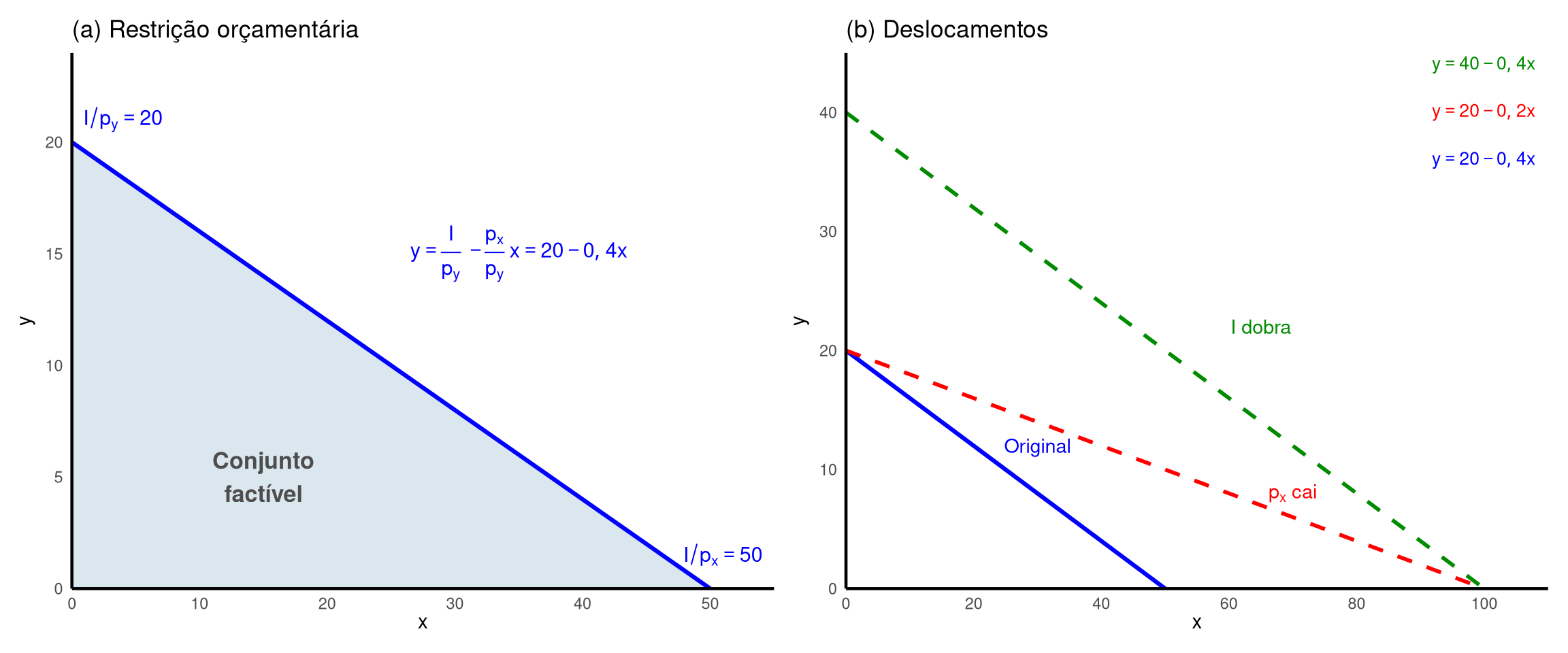
suppressPackageStartupMessages({
  library(ggplot2)
  library(latex2exp)
  library(patchwork)
})

# Painel (a): Restrição orçamentária com conjunto factível
tri_factivel <- data.frame(
  x = c(0, 50, 0),
  y = c(0, 0, 20)
)

p1 <- ggplot() +
  geom_polygon(
    data = tri_factivel,
    aes(x = x, y = y),
    fill = "#b8cfe0", alpha = 0.5
  ) +
  geom_segment(
    aes(x = 0, y = 20, xend = 50, yend = 0),
    color = "blue", linewidth = 1.1
  ) +
  annotate("text", x = 51, y = 1.5,
           label = latex2exp::TeX(r"($I/p_x = 50$)"),
           size = 4, color = "blue") +
  annotate("text", x = 4, y = 21,
           label = latex2exp::TeX(r"($I/p_y = 20$)"),
           size = 4, color = "blue") +
  annotate("text", x = 15, y = 5,
           label = "Conjunto\nfactível",
           size = 4.5, color = "gray30", fontface = "bold") +
  annotate("text", x = 35, y = 15,
           label = latex2exp::TeX(r"($y = \frac{I}{p_y} - \frac{p_x}{p_y} x = 20 - 0{,}4x$)"),
           size = 4, color = "blue") +
  scale_x_continuous(
    expand = c(0, 0),
    limits = c(0, 55),
    breaks = seq(0, 50, 10)
  ) +
  scale_y_continuous(
    expand = c(0, 0),
    limits = c(0, 24),
    breaks = seq(0, 20, 5)
  ) +
  labs(
    x = latex2exp::TeX(r"($x$)"),
    y = latex2exp::TeX(r"($y$)"),
    title = "(a) Restrição orçamentária"
  ) +
  theme_minimal() +
  theme(
    axis.line  = element_line(color = "black", linewidth = 0.8),
    panel.grid = element_blank()
  )

# Painel (b): Deslocamentos
p2 <- ggplot() +
  # Original
  geom_segment(
    aes(x = 0, y = 20, xend = 50, yend = 0),
    color = "blue", linewidth = 1.1
  ) +
  # Renda dobra (I = 200)
  geom_segment(
    aes(x = 0, y = 40, xend = 100, yend = 0),
    color = "green4", linewidth = 1, linetype = "dashed"
  ) +
  # Preço cai (p_x = 1)
  geom_segment(
    aes(x = 0, y = 20, xend = 100, yend = 0),
    color = "red", linewidth = 1, linetype = "dashed"
  ) +
  annotate("text", x = 30, y = 12,
           label = "Original",
           size = 3.8, color = "blue") +
  annotate("text", x = 65, y = 22,
           label = latex2exp::TeX(r"($I$ dobra)"),
           size = 3.8, color = "green4") +
  annotate("text", x = 70, y = 8,
           label = latex2exp::TeX(r"($p_x$ cai)"),
           size = 3.8, color = "red") +
  annotate("text", x = 108, y = 44,
           label = latex2exp::TeX(r"($y = 40 - 0{,}4x$)"),
           size = 3.5, color = "green4", hjust = 1) +
  annotate("text", x = 108, y = 40,
           label = latex2exp::TeX(r"($y = 20 - 0{,}2x$)"),
           size = 3.5, color = "red", hjust = 1) +
  annotate("text", x = 108, y = 36,
           label = latex2exp::TeX(r"($y = 20 - 0{,}4x$)"),
           size = 3.5, color = "blue", hjust = 1) +
  scale_x_continuous(
    expand = c(0, 0),
    limits = c(0, 110),
    breaks = seq(0, 100, 20)
  ) +
  scale_y_continuous(
    expand = c(0, 0),
    limits = c(0, 45),
    breaks = seq(0, 40, 10)
  ) +
  labs(
    x = latex2exp::TeX(r"($x$)"),
    y = latex2exp::TeX(r"($y$)"),
    title = "(b) Deslocamentos"
  ) +
  theme_minimal() +
  theme(
    axis.line  = element_line(color = "black", linewidth = 0.8),
    panel.grid = element_blank()
  )

p1 + p2

Interpretação

A restrição orçamentária define o que é factível, não o que é ótimo. O conjunto factível compreende todas as cestas $(x, y)$ tais que $p_x x + p_y y \leq I$, e a reta orçamentária é a fronteira desse conjunto.

A inclinação $-p_x/p_y$ captura o trade-off de mercado: quantas unidades de $y$ o consumidor deve sacrificar para obter mais uma unidade de $x$. Esse custo de oportunidade independe das preferências do consumidor e é determinado exclusivamente pelos preços relativos.

Mudanças na renda expandem ou contraem as oportunidades de consumo uniformemente (deslocamento paralelo), sem alterar o preço relativo dos bens.

Mudanças nos preços relativos alteram a taxa de troca de mercado (rotação da reta), tornando um bem relativamente mais barato ou mais caro.

O conjunto orçamentário é o ponto de partida da análise: as preferências do consumidor (nos próximos callouts) determinarão qual cesta factível é a melhor. (Nicholson e Snyder, 2012)

Nota 4.2: Maximização da utilidade: caso de dois bens

Símbolo	Significado
$x^, y^$	quantidades ótimas (que maximizam a utilidade)
$TMS = U_x/U_y$	taxa marginal de substituição
$p_x/p_y$	razão de preços (trade-off de mercado)
$TMS = p_x/p_y$	condição de ótimo (tangência)
$U(x,y) = k$	curva de indiferença de nível $k$

Desenvolvimento Teórico

Intuição da tangência (Figura 4.2, Nicholson). O consumidor busca a curva de indiferença mais alta que ainda toque a reta orçamentária. Na Figura 4.2, o ponto $A$ está sobre a reta orçamentária, porém numa curva de indiferença baixa ($U_1$): ao realocar o consumo, é possível atingir uma curva de indiferença superior. O ponto $D$, numa curva mais alta ($U_3$), é inatingível porque está fora do conjunto orçamentário. O ponto $C = (x^*, y^*)$ é aquele em que a curva de indiferença $U_2$ é tangente à reta orçamentária — a melhor cesta acessível.

Condição de primeira ordem. Na tangência, a inclinação da reta orçamentária iguala a inclinação da curva de indiferença:

\[-\frac{p_x}{p_y} = \frac{dy}{dx}\bigg|_{U=k}\]

Como $TMS = -dy/dx|_{U=k} = U_x/U_y$:

\[TMS = \frac{p_x}{p_y}\]

O trade-off psíquico (disposição a substituir) se iguala ao trade-off de mercado (custo de substituir).

Ilustração numérica. Suponha $TMS = 1$ (o consumidor aceita trocar $x$ por $y$ na razão 1:1), mas $p_x/p_y = 2$ (o mercado cobra 2:1). Nesse caso o consumidor valoriza $x$ menos do que o mercado cobra. Reduzindo $x$ em 1 unidade, economiza $p_x$, o que permite comprar $p_x/p_y = 2$ unidades de $y$. Como bastava 1 unidade de $y$ para compensar a perda de 1 unidade de $x$ ($TMS = 1$), a unidade extra de $y$ é um ganho líquido. Esse processo de reajuste continua até que $TMS = p_x/p_y$.

Condições de segunda ordem (Figura 4.3, Nicholson). A tangência é necessária, mas não suficiente. Na Figura 4.3, as curvas de indiferença não obedecem à hipótese de TMS decrescente: o ponto de tangência $C$ é inferior ao ponto $B$ (que não é tangência) e ao ponto $A$ (outra tangência, que é o verdadeiro máximo). Quando a função utilidade é estritamente quase-côncava (TMS decrescente / curvas de indiferença convexas), a tangência é necessária e suficiente Nicholson e Snyder (2012).

Soluções de canto. Às vezes o ótimo ocorre na fronteira: $y = 0$ (ou $x = 0$). Isso acontece quando $TMS > p_x/p_y$ em todos os pontos da reta orçamentária — o consumidor sempre deseja mais $x$ do que a taxa de mercado permite. A condição de primeira ordem torna-se $TMS \geq p_x/p_y$, com igualdade se $y > 0$.

Exercício Resolvido

Problema: encontrar a cesta $(x^*, y^*)$ que maximiza a utilidade do consumidor.

\[\max_{x, y} \; U(x,y) = \sqrt{xy} = (xy)^{1/2} \quad \text{sujeito a} \quad p_x x + p_y y = I\]

com $p_x = 1$, $p_y = 4$, $I = 8$.

Passo 1: escrever a restrição orçamentária

Substituindo os valores na forma geral $p_x x + p_y y = I$:

\[1 \cdot x + 4 \cdot y = 8\]

Isolando $y$:

\[y = \frac{8}{4} - \frac{1}{4}x = 2 - 0{,}25x\]

Passo 2: calcular a TMS

A Taxa Marginal de Substituição é a razão entre as utilidades marginais: $TMS = U_x / U_y$. Para $U(x,y) = (xy)^{1/2} = x^{1/2} y^{1/2}$:

\[\begin{aligned} U_x &= \frac{\partial}{\partial x} \left( x^{1/2} y^{1/2} \right) = \tfrac{1}{2} x^{-1/2} y^{1/2} & & \text{derivada parcial em relação a } x \\[6pt] U_y &= \frac{\partial}{\partial y} \left( x^{1/2} y^{1/2} \right) = \tfrac{1}{2} x^{1/2} y^{-1/2} & & \text{derivada parcial em relação a } y \\[6pt] TMS &= \frac{U_x}{U_y} = \frac{\tfrac{1}{2} x^{-1/2} y^{1/2}}{\tfrac{1}{2} x^{1/2} y^{-1/2}} & & \text{razão das utilidades marginais} \\[6pt] &= \frac{x^{-1/2} y^{1/2}}{x^{1/2} y^{-1/2}} & & \text{cancelando } \tfrac{1}{2} \\[6pt] &= x^{-1/2 - 1/2} \cdot y^{1/2 - (-1/2)} & & \text{regra } a^m / a^n = a^{m-n} \\[6pt] &= x^{-1} \cdot y^{1} = \frac{y}{x} \end{aligned}\]

Para funções Cobb-Douglas $U = x^\alpha y^\beta$, a TMS tem uma fórmula direta: $TMS = \frac{\alpha}{\beta} \cdot \frac{y}{x}$. Como neste caso $\alpha = \beta = 1/2$, a razão $\alpha/\beta = 1$ se cancela, resultando simplesmente em $y/x$.

Passo 3: aplicar a condição de ótimo $TMS = p_x/p_y$

No ponto ótimo, a curva de indiferença tangencia a reta orçamentária, ou seja, suas inclinações se igualam:

\[\begin{aligned} TMS &= \frac{p_x}{p_y} & & \text{condição de tangência} \\[6pt] \frac{y}{x} &= \frac{1}{4} & & \text{substituindo } TMS = y/x \text{ e os preços} \\[6pt] y &= \frac{x}{4} & & \text{isolando } y \end{aligned}\]

Esta equação relaciona $x$ e $y$ no ponto ótimo. Precisamos de uma segunda equação (a restrição orçamentária) para encontrar os valores numéricos.

Passo 4: substituir na restrição orçamentária

Substituindo $y = x/4$ em $x + 4y = 8$:

\[\begin{aligned} x + 4 \cdot \frac{x}{4} &= 8 & & \text{substituindo } y = x/4 \\[6pt] x + x &= 8 & & \text{simplificando} \\[6pt] 2x &= 8 \\[6pt] x^* &= 4 \end{aligned}\]

\[\boxed{x^* = 4}\]

Substituindo $x^* = 4$ na relação de ótimo:

\[\begin{aligned} y^* &= \frac{x^*}{4} = \frac{4}{4} = 1 \end{aligned}\]

\[\boxed{y^* = 1}\]

Passo 5: verificar as condições de ótimo

Condição de tangência: $TMS = y^*/x^* = 1/4 = p_x/p_y$ ✓

Restrição orçamentária: $p_x x^* + p_y y^* = 1 \times 4 + 4 \times 1 = 4 + 4 = 8 = I$ ✓

Utilidade no ótimo: $U(4, 1) = \sqrt{4 \times 1} = \sqrt{4} = 2$

Implementação em R

Código

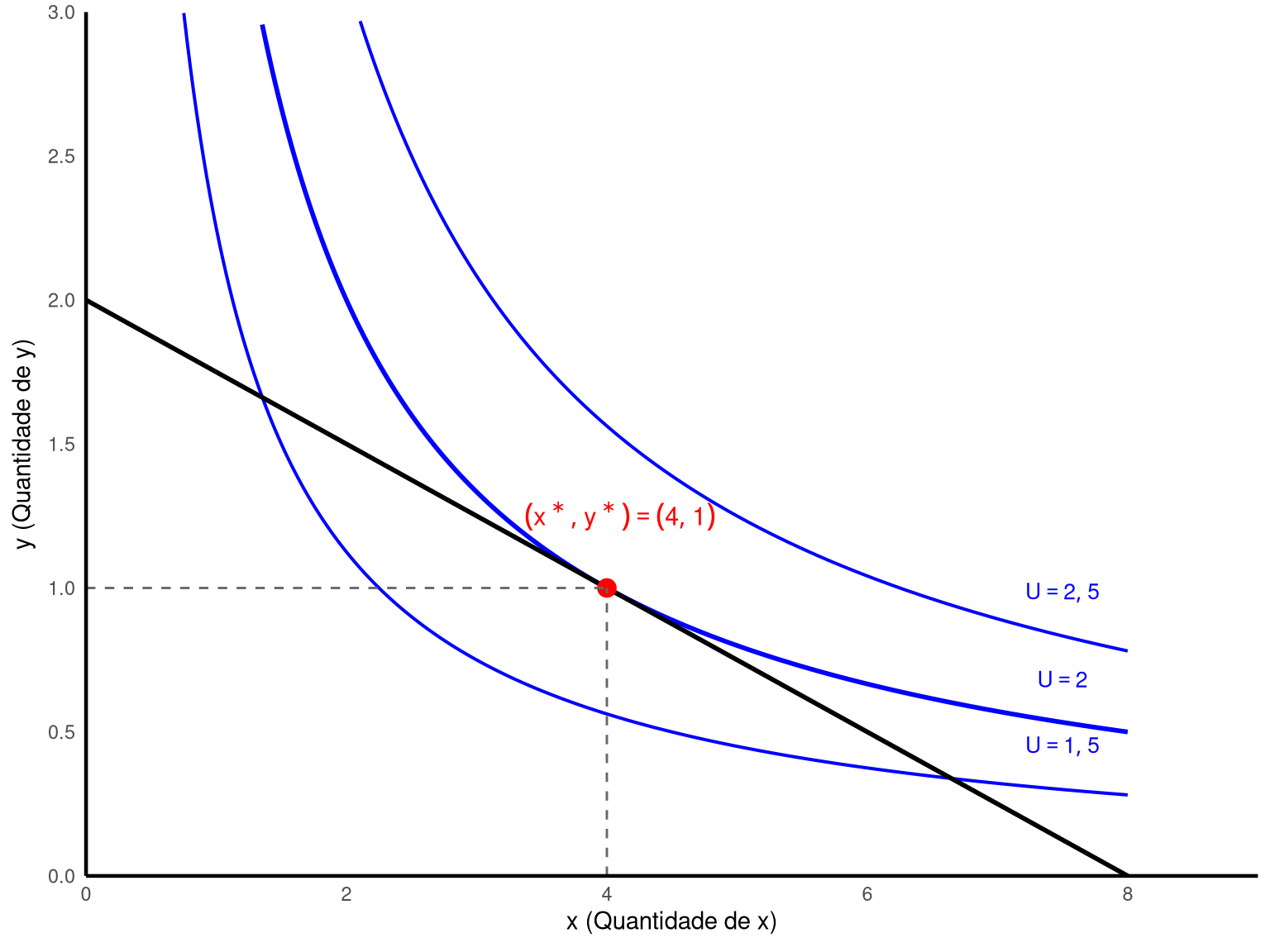
suppressPackageStartupMessages({
  library(ggplot2)
  library(latex2exp)
})

ggplot() +
  # Curvas de indiferença
  geom_function(
    fun = \(x) 2.25 / x,
    xlim = c(0.5, 8), n = 300,
    color = "blue", linewidth = 0.7
  ) +
  geom_function(
    fun = \(x) 4 / x,
    xlim = c(0.5, 8), n = 300,
    color = "blue", linewidth = 1
  ) +
  geom_function(
    fun = \(x) 6.25 / x,
    xlim = c(0.5, 8), n = 300,
    color = "blue", linewidth = 0.7
  ) +
  # Rótulos das curvas de indiferença
  annotate("text", x = 7.5, y = 2.25 / 7.5 + 0.15,
           label = latex2exp::TeX(r"($U = 1{,}5$)"),
           size = 3.5, color = "blue") +
  annotate("text", x = 7.5, y = 4 / 7.5 + 0.15,
           label = latex2exp::TeX(r"($U = 2$)"),
           size = 3.5, color = "blue") +
  annotate("text", x = 7.5, y = 6.25 / 7.5 + 0.15,
           label = latex2exp::TeX(r"($U = 2{,}5$)"),
           size = 3.5, color = "blue") +
  # Reta orçamentária
  geom_segment(
    aes(x = 0, y = 2, xend = 8, yend = 0),
    color = "black", linewidth = 1
  ) +
  # Ponto ótimo
  geom_point(
    aes(x = 4, y = 1),
    color = "red", size = 3.5
  ) +
  # Projeções tracejadas
  geom_segment(
    aes(x = 4, y = 0, xend = 4, yend = 1),
    linetype = "dashed", color = "gray40"
  ) +
  geom_segment(
    aes(x = 0, y = 1, xend = 4, yend = 1),
    linetype = "dashed", color = "gray40"
  ) +
  # Rótulo do ponto ótimo
  annotate("text", x = 4.1, y = 1.25,
           label = latex2exp::TeX(r"($(x^*, y^*) = (4, 1)$)"),
           size = 4, color = "red") +
  scale_x_continuous(
    expand = c(0, 0),
    limits = c(0, 9),
    breaks = c(0, 2, 4, 6, 8)
  ) +
  scale_y_continuous(
    expand = c(0, 0),
    limits = c(0, 3),
    breaks = c(0, 0.5, 1, 1.5, 2, 2.5, 3)
  ) +
  labs(
    x = latex2exp::TeX(r"($x$ (Quantidade de $x$))"),
    y = latex2exp::TeX(r"($y$ (Quantidade de $y$))")
  ) +
  theme_minimal() +
  theme(
    axis.line  = element_line(color = "black", linewidth = 0.8),
    panel.grid = element_blank()
  )

Interpretação

Despesa igual entre os bens: a cesta ótima $(4, 1)$ implica gasto de $p_x x^* = 1 \times 4 = 4$ em $x$ e $p_y y^* = 4 \times 1 = 4$ em $y$. Metade da renda vai para cada bem. Isso não é coincidência — para a Cobb-Douglas $U = x^\alpha y^\beta$ com $\alpha = \beta$, a fração da renda alocada a cada bem é sempre igual: $\frac{\alpha}{\alpha + \beta} = \frac{1}{2}$.

Condição de tangência: no ótimo, $TMS = p_x/p_y = 1/4$. A disposição subjetiva do consumidor a trocar $y$ por $x$ (dada pela TMS) coincide com a taxa objetiva de troca do mercado (dada pela razão de preços). Se $TMS > p_x/p_y$, o consumidor valoriza $x$ mais do que o mercado — compraria mais $x$. Se $TMS < p_x/p_y$, faria o oposto. Somente quando $TMS = p_x/p_y$ não há incentivo para realocar, e a utilidade é máxima.

Leitura inversa: equivalentemente, $p_y/p_x = 4$. Cada unidade de $y$ custa 4 unidades de $x$ no mercado, e o consumidor está disposto a sacrificar exatamente 4 unidades de $x$ por 1 de $y$ — confirmando o equilíbrio.

Este método gráfico funciona bem para dois bens; o método de Lagrange (Note 4.3 e Note 4.4) generaliza o problema para $n$ bens. (Nicholson e Snyder, 2012)

Nota 4.3: Introdução ao método de Lagrange

Revisão: o método de Lagrange

O problema que o método resolve. Frequentemente em economia precisamos otimizar (maximizar ou minimizar) uma função, mas com uma restrição que limita nossas escolhas. Por exemplo:

Maximizar a utilidade do consumidor, mas sem gastar mais do que a renda disponível
Minimizar o custo de produção, mas atingindo um nível mínimo de produto
Maximizar o lucro, mas respeitando restrições de capacidade

Sem restrição, bastaria calcular as derivadas parciais e igualar a zero (otimização livre). Com restrição, precisamos de um método que encontre o ótimo dentro do conjunto permitido pela restrição. O método de Lagrange faz exatamente isso.

A ideia central. Em vez de resolver a restrição para eliminar uma variável e substituir (o que pode ser algebricamente difícil ou impossível), o método incorpora a restrição diretamente na função objetivo por meio de um novo parâmetro $\lambda$ (o multiplicador de Lagrange).

Formulação geral. Considere o problema:

Função objetivo: $f(x, y)$ — o que queremos maximizar ou minimizar
Restrição: $g(x, y) = c$ — a condição que precisa ser satisfeita

Construímos uma nova função, chamada Lagrangiana, que combina a função objetivo com a restrição:

\[\mathscr{L}(x, y, \lambda) = \underbrace{f(x, y)}_{\text{objetivo}} + \underbrace{\lambda\bigl(c - g(x, y)\bigr)}_{\text{restrição incorporada}}\]

Onde:

$\mathscr{L}$ é a função Lagrangiana (uma função de 3 variáveis: $x$, $y$ e $\lambda$)
$\lambda$ é o multiplicador de Lagrange — uma variável nova, cujo valor será determinado junto com $x^*$ e $y^*$
O termo $c - g(x, y)$ é a restrição reescrita como $= 0$

Note que quando a restrição é satisfeita ($g(x,y) = c$), o termo $\lambda(c - g(x,y)) = 0$, e a Lagrangiana se reduz à função objetivo $f(x,y)$. O multiplicador $\lambda$ “penaliza” desvios da restrição.

Etapas do método:

Identificar $f(x,y)$ (objetivo), $g(x,y)$ (restrição) e $c$ (valor da restrição)
Construir a Lagrangiana: $\mathscr{L} = f(x,y) + \lambda(c - g(x,y))$
Calcular as três derivadas parciais e igualar cada uma a zero. Essas equações são chamadas de Condições de Primeira Ordem (CPOs), são as condições necessárias para que o ponto seja um ótimo:

\[\frac{\partial \mathscr{L}}{\partial x} = 0 \qquad \text{(CPO em } x \text{)}\]

\[\frac{\partial \mathscr{L}}{\partial y} = 0 \qquad \text{(CPO em } y \text{)}\]

\[\frac{\partial \mathscr{L}}{\partial \lambda} = 0 \qquad \text{(recupera a restrição original)}\]

Resolver o sistema de 3 equações e 3 incógnitas ($x^*$, $y^*$, $\lambda$)
Interpretar $\lambda$: mede o ganho (ou custo) marginal de relaxar a restrição em uma unidade

Exemplo rápido. Maximizar $f(x, y) = xy$ sujeito a $x + y = 10$.

Etapa 1: identificar as funções. Aqui $f(x,y) = xy$ é a função a maximizar, $g(x,y) = x + y$ é a restrição, e $c = 10$.

Etapa 2: construir a Lagrangiana. Substituindo na fórmula $\mathscr{L} = f(x,y) + \lambda(c - g(x,y))$:

\[\mathscr{L}(x, y, \lambda) = xy + \lambda(10 - x - y)\]

Etapa 3: calcular as derivadas parciais (CPOs) e igualar a zero.

A Lagrangiana é $\mathscr{L} = \underbrace{xy}_{\text{termo 1}} + \underbrace{\lambda(10 - x - y)}_{\text{termo 2}}$. Derivamos em relação a cada variável separadamente.

Derivada em relação a $x$ (tratar $y$ e $\lambda$ como constantes):

\[\begin{aligned} \frac{\partial \mathscr{L}}{\partial x} &= \frac{\partial(xy)}{\partial x} + \frac{\partial[\lambda(10 - x - y)]}{\partial x} & & \text{derivada da soma = soma das derivadas} \\[6pt] &= y + \lambda \cdot (-1) & & \frac{\partial(xy)}{\partial x} = y \text{; } \frac{\partial(-x)}{\partial x} = -1 \text{; os demais termos são constantes} \\[6pt] &= y - \lambda = 0 & & \text{igualando a zero (CPO)} \end{aligned}\]

\[\Rightarrow \quad y = \lambda \qquad \text{(equação 1)}\]

Derivada em relação a $y$ (tratar $x$ e $\lambda$ como constantes):

\[\begin{aligned} \frac{\partial \mathscr{L}}{\partial y} &= \frac{\partial(xy)}{\partial y} + \frac{\partial[\lambda(10 - x - y)]}{\partial y} & & \text{derivada da soma} \\[6pt] &= x + \lambda \cdot (-1) & & \frac{\partial(xy)}{\partial y} = x \text{; } \frac{\partial(-y)}{\partial y} = -1 \\[6pt] &= x - \lambda = 0 & & \text{igualando a zero (CPO)} \end{aligned}\]

\[\Rightarrow \quad x = \lambda \qquad \text{(equação 2)}\]

Derivada em relação a $\lambda$ (tratar $x$ e $y$ como constantes):

\[\begin{aligned} \frac{\partial \mathscr{L}}{\partial \lambda} &= \frac{\partial(xy)}{\partial \lambda} + \frac{\partial[\lambda(10 - x - y)]}{\partial \lambda} & & \text{derivada da soma} \\[6pt] &= 0 + (10 - x - y) & & xy \text{ não depende de } \lambda \text{; } \frac{\partial(\lambda \cdot k)}{\partial \lambda} = k \\[6pt] &= 10 - x - y = 0 & & \text{igualando a zero (recupera a restrição)} \end{aligned}\]

\[\Rightarrow \quad x + y = 10 \qquad \text{(equação 3)}\]

Etapa 4: resolver o sistema.

Temos 3 equações e 3 incógnitas ($x$, $y$, $\lambda$):

\[\begin{cases} y = \lambda & \text{(equação 1)} \\ x = \lambda & \text{(equação 2)} \\ x + y = 10 & \text{(equação 3)} \end{cases}\]

Das equações 1 e 2, observamos que $y = \lambda$ e $x = \lambda$, portanto $x = y$. Ambas as variáveis são iguais a $\lambda$.

Substituindo $x = \lambda$ e $y = \lambda$ na equação 3:

\[\begin{aligned} x + y &= 10 & & \text{equação 3} \\[6pt] \lambda + \lambda &= 10 & & \text{substituindo } x = \lambda \text{ e } y = \lambda \\[6pt] 2\lambda &= 10 & & \text{somando} \\[6pt] \lambda &= \frac{10}{2} = 5 & & \text{dividindo ambos os lados por 2} \end{aligned}\]

Com $\lambda = 5$, recuperamos os valores ótimos:

\[\begin{aligned} x^* &= \lambda = 5 \\[6pt] y^* &= \lambda = 5 \end{aligned}\]

\[\boxed{x^* = 5, \qquad y^* = 5}\]

Valor ótimo da função objetivo:

\[f(x^*, y^*) = f(5,\; 5) = 5 \times 5 = 25\]

Verificação da restrição:

\[x^* + y^* = 5 + 5 = 10 = c \quad \checkmark\]

A restrição é satisfeita, confirmando que a solução é viável.

Interpretação de $\lambda$.

O multiplicador $\lambda = 5$ mede o ganho marginal de relaxar a restrição: se dispuséssemos de uma unidade a mais de recurso (passando de $x + y = 10$ para $x + y = 11$), o valor ótimo de $f$ aumentaria em aproximadamente $\lambda = 5$.

Podemos verificar resolvendo o novo problema ($x + y = 11$):

\[x^* = y^* = \frac{11}{2} = 5{,}5\]

\[f(5{,}5;\; 5{,}5) = 5{,}5 \times 5{,}5 = 30{,}25\]

A variação no valor ótimo:

\[\Delta f = 30{,}25 - 25 = 5{,}25 \approx \lambda = 5\]

A aproximação não é exata porque $\lambda$ mede a variação marginal (para mudanças infinitesimais na restrição), e aqui a mudança foi discreta ($\Delta c = 1$). Para mudanças menores, a aproximação melhora.

Agora aplicamos esse método a um problema econômico concreto.

Exemplo: ingressos de futebol e cinema

Baseado em Baidya, Aiube e Mendes (2014, p. 254, Exemplo 7.7).

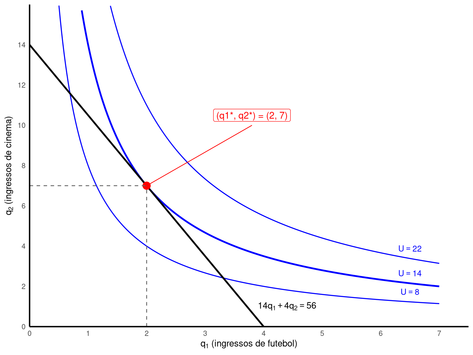
Enunciado. Suponha que a sua função utilidade seja $U(q_1, q_2) = q_1 q_2$, onde $q_1$ é a quantidade de ingressos para o futebol e $q_2$ a quantidade de ingressos para o cinema. O preço do ingresso de cinema é $p_2 = 4$ e do futebol $p_1 = 14$. Sua renda de $I = 56$ será toda empregada na compra de ingressos. Que quantidade de cada ingresso você irá adquirir?

Formulação do problema:

\[\max_{q_1, q_2} \; U(q_1, q_2) = q_1 q_2 \quad \text{sujeito a} \quad 14 q_1 + 4 q_2 = 56\]

Passo 1: montar o Lagrangiano

Identificando: $f(q_1, q_2) = q_1 q_2$ (objetivo), $g(q_1, q_2) = 14 q_1 + 4 q_2$ (restrição), $c = 56$.

\[\mathscr{L}(q_1, q_2, \lambda) = q_1 q_2 + \lambda(56 - 14 q_1 - 4 q_2)\]

Passo 2: condições de primeira ordem

Derivada em relação a $q_1$ (tratar $q_2$ e $\lambda$ como constantes):

\[\begin{aligned} \frac{\partial \mathscr{L}}{\partial q_1} &= \frac{\partial}{\partial q_1}\bigl[q_1 q_2 + \lambda(56 - 14 q_1 - 4 q_2)\bigr] & & \text{Lagrangiana completa} \\[6pt] &= \frac{\partial(q_1 q_2)}{\partial q_1} + \lambda \cdot \frac{\partial(56 - 14 q_1 - 4 q_2)}{\partial q_1} & & \text{derivada da soma = soma das derivadas} \\[6pt] &= q_2 + \lambda \cdot (-14) & & \text{derivada de } q_1 q_2 \text{ em } q_1 \text{ é } q_2 \text{; derivada de } {-14 q_1} \text{ é } {-14} \\[6pt] &= q_2 - 14\lambda = 0 & & \text{igualando a zero (CPO)} \end{aligned}\]

\[\Rightarrow \quad q_2 = 14\lambda \qquad \text{(CPO 1)}\]

Derivada em relação a $q_2$ (tratar $q_1$ e $\lambda$ como constantes):

\[\begin{aligned} \frac{\partial \mathscr{L}}{\partial q_2} &= \frac{\partial}{\partial q_2}\bigl[q_1 q_2 + \lambda(56 - 14 q_1 - 4 q_2)\bigr] & & \text{Lagrangiana completa} \\[6pt] &= \frac{\partial(q_1 q_2)}{\partial q_2} + \lambda \cdot \frac{\partial(56 - 14 q_1 - 4 q_2)}{\partial q_2} & & \text{derivada da soma} \\[6pt] &= q_1 + \lambda \cdot (-4) & & \text{derivada de } q_1 q_2 \text{ em } q_2 \text{ é } q_1 \text{; derivada de } {-4 q_2} \text{ é } {-4} \\[6pt] &= q_1 - 4\lambda = 0 & & \text{igualando a zero (CPO)} \end{aligned}\]

\[\Rightarrow \quad q_1 = 4\lambda \qquad \text{(CPO 2)}\]

Derivada em relação a $\lambda$ (recupera a restrição original):

\[\begin{aligned} \frac{\partial \mathscr{L}}{\partial \lambda} &= \frac{\partial}{\partial \lambda}\bigl[q_1 q_2 + \lambda(56 - 14 q_1 - 4 q_2)\bigr] & & \text{Lagrangiana completa} \\[6pt] &= 0 + (56 - 14 q_1 - 4 q_2) & & q_1 q_2 \text{ não depende de } \lambda \text{; derivada de } \lambda(\cdot) \text{ é } (\cdot) \\[6pt] &= 56 - 14 q_1 - 4 q_2 = 0 & & \text{igualando a zero (CPO)} \end{aligned}\]

\[\Rightarrow \quad 14 q_1 + 4 q_2 = 56 \qquad \text{(CPO 3)}\]

Passo 3: resolver o sistema

Temos 3 equações e 3 incógnitas ($q_1$, $q_2$, $\lambda$):

\[\begin{cases} q_2 = 14\lambda & \text{(CPO 1)} \\ q_1 = 4\lambda & \text{(CPO 2)} \\ 14 q_1 + 4 q_2 = 56 & \text{(CPO 3)} \end{cases}\]

Das CPOs 1 e 2, já temos $q_1$ e $q_2$ em função de $\lambda$. Substituindo na CPO 3:

\[\begin{aligned} 14 \cdot (4\lambda) + 4 \cdot (14\lambda) &= 56 & & \text{substituindo } q_1 = 4\lambda \text{ e } q_2 = 14\lambda \\[6pt] 56\lambda + 56\lambda &= 56 & & \text{multiplicando} \\[6pt] 112\lambda &= 56 & & \text{somando os termos em } \lambda \\[6pt] \lambda &= \frac{56}{112} = \frac{1}{2} = 0{,}5 & & \text{dividindo ambos os lados por } 112 \end{aligned}\]

Com $\lambda = 0{,}5$, encontramos as quantidades ótimas:

\[\begin{aligned} q_1^* &= 4\lambda = 4 \times 0{,}5 = 2 & & \text{(ingressos de futebol)} \\[6pt] q_2^* &= 14\lambda = 14 \times 0{,}5 = 7 & & \text{(ingressos de cinema)} \end{aligned}\]

\[\boxed{q_1^* = 2 \text{ (futebol)}, \qquad q_2^* = 7 \text{ (cinema)} }\]

Passo 4: verificações

Restrição orçamentária:

\[p_1 q_1^* + p_2 q_2^* = 14 \times 2 + 4 \times 7 = 28 + 28 = 56 = I \quad \checkmark\]

Note que o consumidor gasta metade da renda ($28) em cada bem. Isso ocorre porque $U = q_1 q_2$ é uma Cobb-Douglas com expoentes iguais ($\alpha = \beta = 1$, ou equivalentemente, após normalização, $\alpha = \beta = 0{,}5$), implicando frações da renda iguais.

Condição de ótimo ($TMS = p_1/p_2$):

Calculamos a TMS no ponto ótimo usando a razão das utilidades marginais:

\[\begin{aligned} TMS &= \frac{U_{q_1}}{U_{q_2}} & & \text{definição} \\[6pt] &= \frac{\partial(q_1 q_2)/\partial q_1}{\partial(q_1 q_2)/\partial q_2} & & \text{substituindo } U = q_1 q_2 \\[6pt] &= \frac{q_2}{q_1} & & \text{derivada de } q_1 q_2 \text{ em } q_1 \text{ é } q_2 \text{; em } q_2 \text{ é } q_1 \\[6pt] &= \frac{7}{2} = 3{,}5 & & \text{substituindo } q_1^* = 2, \; q_2^* = 7 \end{aligned}\]

Comparando com a razão de preços:

\[\frac{p_1}{p_2} = \frac{14}{4} = 3{,}5 = TMS \quad \checkmark\]

O consumidor está disposto a trocar 3,5 ingressos de cinema por 1 de futebol, e o mercado cobra exatamente essa taxa.

Utilidade no ótimo:

\[\begin{aligned} U(q_1^*, q_2^*) &= U(2,\; 7) & & \text{substituindo os valores ótimos} \\[6pt] &= 2 \times 7 = 14 & & \text{aplicando } U = q_1 q_2 \end{aligned}\]

Interpretação de $\lambda = 0{,}5$:

Cada real adicional de renda aumentaria a utilidade em aproximadamente $\lambda = 0{,}5$. Podemos verificar: se a renda passasse de $I = 56$ para $I = 57$ ($\Delta I = 1$), basta resolver o mesmo sistema de CPOs com a nova renda:

\[\begin{aligned} 112\lambda &= 57 & & \text{mesma estrutura do Passo 3, com } I = 57 \\[6pt] \lambda &= \frac{57}{112} \approx 0{,}5089 \\[6pt] q_1^* &= 4\lambda = 4 \times \frac{57}{112} = \frac{57}{28} \approx 2{,}036 & & \text{usando CPO 2: } q_1 = 4\lambda \\[6pt] q_2^* &= 14\lambda = 14 \times \frac{57}{112} = \frac{57}{8} = 7{,}125 & & \text{usando CPO 1: } q_2 = 14\lambda \end{aligned}\]

A nova utilidade e a variação:

\[\begin{aligned} U' &= 2{,}036 \times 7{,}125 \approx 14{,}506 & & \text{nova utilidade} \\[6pt] \Delta U &= 14{,}506 - 14 = 0{,}506 & & \text{variação} \\[6pt] \lambda \times \Delta I &= 0{,}5 \times 1 = 0{,}5 \approx \Delta U & & \checkmark \end{aligned}\]

Implementação em R

Código

suppressPackageStartupMessages({
  library(ggplot2)
  library(latex2exp)
})

# Parâmetros
p1 <- 14; p2 <- 4; I_val <- 56
q1_star <- 2; q2_star <- 7
U_star <- q1_star * q2_star  # = 14

ggplot() +
  # Curvas de indiferença: U = q1 * q2 => q2 = U/q1
  geom_function(
    fun = \(q1) 8 / q1,
    xlim = c(0.3, 7), n = 300,
    color = "blue", linewidth = 0.6
  ) +
  geom_function(
    fun = \(q1) 14 / q1,
    xlim = c(0.5, 7), n = 300,
    color = "blue", linewidth = 1
  ) +
  geom_function(
    fun = \(q1) 22 / q1,
    xlim = c(0.8, 7), n = 300,
    color = "blue", linewidth = 0.6
  ) +
  # Rótulos das CIs
  annotate("text", x = 6.5, y = 8 / 6.5 + 0.5,
           label = TeX(r"($U = 8$)"),
           size = 3.5, color = "blue") +
  annotate("text", x = 6.5, y = 14 / 6.5 + 0.5,
           label = TeX(r"($U = 14$)"),
           size = 3.5, color = "blue") +
  annotate("text", x = 6.5, y = 22 / 6.5 + 0.5,
           label = TeX(r"($U = 22$)"),
           size = 3.5, color = "blue") +
  # Reta orçamentária: 14q1 + 4q2 = 56 => q2 = 14 - 3.5*q1
  geom_segment(
    aes(x = 0, y = I_val / p2, xend = I_val / p1, yend = 0),
    color = "black", linewidth = 1
  ) +
  # Rótulo da reta orçamentária (próximo ao eixo X)
  annotate("text", x = 4.4, y = 1,
           label = TeX(r"($14q_1 + 4q_2 = 56$)"),
           size = 3.8, color = "black") +
  # Ponto ótimo
  geom_point(
    aes(x = q1_star, y = q2_star),
    color = "red", size = 4
  ) +
  # Projeções tracejadas
  geom_segment(
    aes(x = q1_star, y = 0, xend = q1_star, yend = q2_star),
    linetype = "dashed", color = "gray40"
  ) +
  geom_segment(
    aes(x = 0, y = q2_star, xend = q1_star, yend = q2_star),
    linetype = "dashed", color = "gray40"
  ) +
  # Linha conectando o ponto ótimo ao rótulo
  geom_segment(
    aes(x = q1_star, y = q2_star, xend = 3.8, yend = 10),
    color = "red", linewidth = 0.4
  ) +
  # Rótulo do ponto ótimo
  annotate("label", x = 3.8, y = 10.5,
           label = "(q1*, q2*) = (2, 7)",
           size = 4, color = "red",
           fill = "white", label.size = 0.3) +
  scale_x_continuous(
    expand = c(0, 0),
    limits = c(0, 7.5),
    breaks = 0:7
  ) +
  scale_y_continuous(
    expand = c(0, 0),
    limits = c(0, 16),
    breaks = seq(0, 14, 2)
  ) +
  labs(
    x = TeX(r"($q_1$ (ingressos de futebol))"),
    y = TeX(r"($q_2$ (ingressos de cinema))")
  ) +
  theme_minimal() +
  theme(
    axis.line  = element_line(color = "black", linewidth = 0.8),
    panel.grid = element_blank()
  )

Interpretação

O consumidor compra 2 ingressos de futebol e 7 ingressos de cinema: como futebol é 3,5 vezes mais caro que cinema, a quantidade ótima de cinema é 3,5 vezes maior que a de futebol.
A despesa é dividida igualmente: R$28 em futebol e R$28 em cinema. Isso é consequência direta da Cobb-Douglas com expoentes iguais (frações da renda de 50% cada).
No gráfico, o ponto ótimo $(2, 7)$ está na curva $U = 14$, que é a curva de indiferença mais alta que toca a reta orçamentária. As curvas $U = 8$ e $U = 22$ são, respectivamente, acessível (mas subótima) e inacessível.

Nota 4.4: O caso geral: Lagrangiano para $n$ bens

No callout anterior, resolvemos um exemplo concreto com $U = q_1 q_2$, preços numéricos e renda fixa. Agora generalizamos o método para $n$ bens com preços e renda quaisquer, extraindo os resultados fundamentais da teoria do consumidor.

Símbolo	Significado
$\mathscr{L}$	função Lagrangiana
$\lambda$	multiplicador de Lagrange
$U_i = \partial U/\partial x_i$	utilidade marginal do bem $i$
$\partial \mathscr{L}/\partial x_i = 0$	condição de primeira ordem (CPO) para o bem $i$
$U_i/p_i = \lambda$	utilidade marginal por real gasto deve ser igual para todos os bens

O problema

O consumidor deseja maximizar a função utilidade $U(x_1, x_2, \ldots, x_n)$ sujeita à restrição orçamentária:

\[I = p_1 x_1 + p_2 x_2 + \cdots + p_n x_n\]

Isto é, escolher as quantidades $x_1, x_2, \ldots, x_n$ que maximizam a satisfação sem exceder a renda disponível $I$ (Eq. 4.4–4.6 Nicholson).

Montagem do Lagrangiano

\[\mathscr{L} = U(x_1, x_2, \ldots, x_n) + \lambda(I - p_1 x_1 - p_2 x_2 - \cdots - p_n x_n)\]

Compare com o exemplo anterior: lá tínhamos $\mathscr{L} = q_1 q_2 + \lambda(56 - 14q_1 - 4q_2)$. Aqui, $U$ e os preços são genéricos, mas a estrutura é idêntica.

Condições de primeira ordem (CPOs)

Tomando as derivadas parciais e igualando a zero (mesma mecânica do exemplo anterior):

\[\begin{aligned} \frac{\partial \mathscr{L}}{\partial x_1} &= \frac{\partial U}{\partial x_1} - \lambda p_1 = 0 & & \text{CPO do bem 1} \\[6pt] \frac{\partial \mathscr{L}}{\partial x_2} &= \frac{\partial U}{\partial x_2} - \lambda p_2 = 0 & & \text{CPO do bem 2} \\[6pt] &\;\;\vdots \\[6pt] \frac{\partial \mathscr{L}}{\partial x_n} &= \frac{\partial U}{\partial x_n} - \lambda p_n = 0 & & \text{CPO do bem } n \\[6pt] \frac{\partial \mathscr{L}}{\partial \lambda} &= I - p_1 x_1 - p_2 x_2 - \cdots - p_n x_n = 0 & & \text{restrição orçamentária} \end{aligned}\]

Essas $n + 1$ equações podem ser resolvidas para as $n + 1$ incógnitas: $x_1^*, x_2^*, \ldots, x_n^*$ e $\lambda$.

Implicações das CPOs

Implicação 1: TMS = razão de preços. Dividindo duas CPOs quaisquer $i$ e $j$:

\[\begin{aligned} \frac{U_i - \lambda p_i}{U_j - \lambda p_j} &= \frac{0}{0} & & \text{ambas CPOs iguais a zero} \\[6pt] \frac{U_i}{U_j} &= \frac{p_i}{p_j} & & \text{dividindo } U_i = \lambda p_i \text{ por } U_j = \lambda p_j \\[6pt] TMS(x_i \text{ por } x_j) &= \frac{p_i}{p_j} & & \text{condição de tangência generalizada} \end{aligned}\]

Esta é a mesma condição de tangência do caso de dois bens, agora generalizada para qualquer par de bens. No exemplo anterior, encontramos $q_2/q_1 = p_1/p_2 = 14/4 = 3{,}5$ — um caso particular desta regra geral.

Implicação 2: utilidade marginal por real gasto é igual para todos os bens.

De cada CPO podemos isolar $\lambda$:

\[\begin{aligned} U_i &= \lambda p_i & & \text{CPO do bem } i \\[6pt] \lambda &= \frac{U_i}{p_i} & & \text{isolando } \lambda \end{aligned}\]

A fração $U_i / p_i$ tem uma interpretação direta: é a utilidade adicional obtida por real gasto no bem $i$. Se o bem 1 custa $p_1 = 4$ reais e cada unidade adicional dá $U_1 = 2$ de utilidade, então cada real gasto nesse bem rende $2/4 = 0{,}5$ de utilidade.

Como $\lambda$ é o mesmo para todas as CPOs:

\[\begin{aligned} \lambda &= \frac{U_1}{p_1} = \frac{U_2}{p_2} = \cdots = \frac{U_n}{p_n} & & \text{equalização marginal} \end{aligned}\]

No ótimo, todo bem consumido rende a mesma utilidade por real gasto. Se um bem oferecesse mais utilidade por real que outro, o consumidor realocaria seus gastos em direção a ele (comprando mais desse bem e menos do outro), até que os retornos marginais se equalizassem.

Exemplo: suponha que no ponto atual $\frac{U_1}{p_1} = 3$ e $\frac{U_2}{p_2} = 1$. O bem 1 rende 3 vezes mais utilidade por real que o bem 2. O consumidor deveria transferir gastos do bem 2 para o bem 1. Ao comprar mais do bem 1, sua utilidade marginal $U_1$ cai (utilidade marginal decrescente); ao comprar menos do bem 2, $U_2$ sobe. O ajuste continua até $U_1/p_1 = U_2/p_2$.

Interpretação do multiplicador $\lambda$

$\lambda$ é a utilidade marginal da renda: a utilidade extra que o consumidor obtém se sua renda aumentar em um real. Assim como no exemplo rápido (onde $\lambda = 5$ media o ganho de relaxar $x + y = 10$) e no exemplo do futebol/cinema (onde $\lambda = 0{,}5$ media o ganho de um real a mais de renda), aqui $\lambda$ mede o valor (em utilidade) de um real a mais de renda no caso geral.

Isso leva a uma reescrita importante das CPOs:

\[\begin{aligned} U_i &= \lambda p_i & & \text{CPO do bem } i \\[6pt] p_i &= \frac{U_i}{\lambda} & & \text{preço = disposição a pagar} \end{aligned}\]

O preço do bem $i$ é igual à sua utilidade marginal dividida pela utilidade marginal da renda. Na margem, o preço reflete a disposição do consumidor a pagar por mais uma unidade. Isso é fundamental na economia do bem-estar: a disposição a pagar pode ser inferida dos preços de mercado Nicholson e Snyder (2012).

Soluções de canto (condições de Kuhn-Tucker)

Até aqui, assumimos que o consumidor compra quantidades positivas de todos os bens (solução interior). Mas e se o ótimo for não consumir algum bem? Por exemplo, um vegetariano que não compra carne ($x_{\text{carne}} = 0$). Nesse caso, as CPOs com igualdade estrita não se aplicam, e precisamos das condições de Kuhn-Tucker.

O problema: nas CPOs interiores, exigimos $\frac{\partial U}{\partial x_i} - \lambda p_i = 0$. Mas se o consumidor gostaria de consumir $x_i < 0$ (o que não é possível), a melhor opção é $x_i = 0$. Nesse ponto, a derivada da Lagrangiana pode ser negativa em vez de zero.

As condições de Kuhn-Tucker generalizam as CPOs para permitir $x_i = 0$:

\[\frac{\partial U}{\partial x_i} - \lambda p_i \leq 0 \qquad (i = 1, \ldots, n)\]

com a regra de folga complementar:

Se $\frac{\partial U}{\partial x_i} - \lambda p_i = 0$, então $x_i \geq 0$ (pode ser positivo — solução interior)
Se $\frac{\partial U}{\partial x_i} - \lambda p_i < 0$, então $x_i = 0$ (solução de canto)

Interpretação econômica. Rearranjando a desigualdade:

\[\begin{aligned} U_i - \lambda p_i &\leq 0 & & \text{condição de Kuhn-Tucker} \\[6pt] U_i &\leq \lambda p_i & & \text{somando } \lambda p_i \\[6pt] \frac{U_i}{\lambda} &\leq p_i & & \text{dividindo por } \lambda \end{aligned}\]

O lado esquerdo é a disposição a pagar do consumidor pelo bem $i$ (a utilidade marginal do bem convertida em reais, dividindo pela utilidade marginal da renda $\lambda$). O lado direito é o preço de mercado.

Se $\frac{U_i}{\lambda} = p_i$: a disposição a pagar iguala o preço → o consumidor compra o bem ($x_i > 0$)
Se $\frac{U_i}{\lambda} < p_i$: a disposição a pagar é menor que o preço → o bem é “caro demais” e o consumidor não compra ($x_i = 0$)

Isso é intuitivo: ninguém compra um bem cujo preço excede o valor que ele atribui à primeira unidade Nicholson e Snyder (2012), Jehle e Reny (2011).

Exercício resolvido

Problema: encontrar as funções de demanda para $U(x, y) = x^{0{,}5} y^{0{,}5}$ com preços genéricos $p_x$, $p_y$ e renda $I$.

\[\max_{x, y} \; U(x,y) = x^{0{,}5} y^{0{,}5} \quad \text{sujeito a} \quad p_x x + p_y y = I\]

Passo 1: montar o Lagrangiano

Identificando as funções: $f(x,y) = x^{0{,}5} y^{0{,}5}$ (objetivo), $g(x,y) = p_x x + p_y y$ (restrição), $c = I$. Substituindo na fórmula $\mathscr{L} = f + \lambda(c - g)$:

\[\mathscr{L} = x^{0{,}5} y^{0{,}5} + \lambda(I - p_x x - p_y y)\]

Passo 2: Condições de primeira ordem.

\[\begin{aligned} \frac{\partial \mathscr{L}}{\partial x} &= 0{,}5\, x^{-0{,}5} y^{0{,}5} - \lambda p_x = 0 & & \text{(CPO 1): regra da potência em } x, \text{ mantendo } y^{0{,}5} \\[6pt] \frac{\partial \mathscr{L}}{\partial y} &= 0{,}5\, x^{0{,}5} y^{-0{,}5} - \lambda p_y = 0 & & \text{(CPO 2): regra da potência em } y, \text{ mantendo } x^{0{,}5} \\[6pt] \frac{\partial \mathscr{L}}{\partial \lambda} &= I - p_x x - p_y y = 0 & & \text{(CPO 3): restrição orçamentária} \end{aligned}\]

Temos 3 equações e 3 incógnitas ($x$, $y$, $\lambda$).

Passo 3: Dividir CPO 1 pela CPO 2 para eliminar $\lambda$.

\[\begin{aligned} \frac{0{,}5\, x^{-0{,}5} y^{0{,}5}}{0{,}5\, x^{0{,}5} y^{-0{,}5}} &= \frac{\lambda p_x}{\lambda p_y} & & \text{dividindo CPO 1 pela CPO 2} \\[6pt] \frac{x^{-0{,}5} y^{0{,}5}}{x^{0{,}5} y^{-0{,}5}} &= \frac{p_x}{p_y} & & \text{cancelando } 0{,}5 \text{ e } \lambda \\[6pt] x^{-0{,}5 - 0{,}5} \cdot y^{0{,}5 -(-0{,}5)} &= \frac{p_x}{p_y} & & \text{regra } a^m / a^n = a^{m-n} \\[6pt] x^{-1} \cdot y^{1} &= \frac{p_x}{p_y} \\[6pt] \frac{y}{x} &= \frac{p_x}{p_y} & & \text{TMS = razão de preços} \\[6pt] p_y y &= p_x x & & \text{multiplicando ambos os lados por } x \cdot p_y \end{aligned}\]

No ótimo, a despesa com $y$ é igual à despesa com $x$. Isso ocorre porque os expoentes da Cobb-Douglas são iguais ($0{,}5$ e $0{,}5$), implicando que o consumidor divide sua renda igualmente entre os dois bens.

Passo 4: Substituir na restrição orçamentária.

Do Passo 3 temos $p_y y = p_x x$; da CPO 3, $p_x x + p_y y = I$. Substituindo:

\[\begin{aligned} p_x x + \underbrace{p_y y}_{= p_x x} &= I & & \text{substituindo } p_y y = p_x x \\[6pt] 2 p_x x &= I \\[6pt] x^* &= \frac{I}{2 p_x} \end{aligned}\]

\[\boxed{x^* = \frac{I}{2 p_x}}\]

Para $y^*$, substituímos $x^*$ na relação $p_y y = p_x x$:

\[\begin{aligned} p_y y &= p_x \cdot \frac{I}{2p_x} = \frac{I}{2} & & \text{substituindo } x^* \\[6pt] y^* &= \frac{I}{2 p_y} \end{aligned}\]

\[\boxed{y^* = \frac{I}{2 p_y}}\]

Essas são as funções de demanda: expressam as quantidades ótimas em termos dos parâmetros do problema ($p_x$, $p_y$, $I$). Este resultado é um caso particular ($\alpha = \beta = 0{,}5$) da demanda marshalliana Cobb-Douglas, que será derivada para expoentes genéricos no Note 4.5.

Passo 5: Calcular $\lambda$.

Isolando $\lambda$ na CPO 1 e substituindo $x^*$ e $y^*$:

\[\begin{aligned} \lambda &= \frac{0{,}5\, x^{-0{,}5} y^{0{,}5}}{p_x} & & \text{isolando } \lambda \text{ na CPO 1} \\[6pt] &= \frac{0{,}5}{p_x} \cdot \left(\frac{I}{2p_x}\right)^{-0{,}5} \cdot \left(\frac{I}{2p_y}\right)^{0{,}5} & & \text{substituindo } x^* \text{ e } y^* \\[6pt] &= \frac{0{,}5}{p_x} \cdot \frac{\sqrt{2p_x}}{\sqrt{I}} \cdot \frac{\sqrt{I}}{\sqrt{2p_y}} & & a^{-0{,}5} = 1/\sqrt{a}, \;\; a^{0{,}5} = \sqrt{a} \\[6pt] &= \frac{0{,}5}{p_x} \cdot \sqrt{\frac{p_x}{p_y}} & & \text{cancelando } \sqrt{I} \text{ e } \sqrt{2} \\[6pt] &= \frac{0{,}5}{\sqrt{p_x} \cdot \sqrt{p_y}} & & p_x = \sqrt{p_x} \cdot \sqrt{p_x} \\[6pt] &= \frac{1}{2\sqrt{p_x p_y}} \end{aligned}\]

\[\boxed{\lambda = \frac{1}{2\sqrt{p_x p_y}} }\]

Passo 6: Verificação numérica com $p_x = 1$, $p_y = 4$, $I = 8$.

As fórmulas genéricas são válidas para quaisquer valores. Verificando:

\[\begin{aligned} x^* &= \frac{I}{2 p_x} = \frac{8}{2 \times 1} = 4 & & \text{demanda marshalliana de } x \\[6pt] y^* &= \frac{I}{2 p_y} = \frac{8}{2 \times 4} = 1 & & \text{demanda marshalliana de } y \end{aligned}\]

Verificação 1: restrição orçamentária.

\[\begin{aligned} p_x x^* + p_y y^* &= 1 \times 4 + 4 \times 1 = 8 = I \quad \checkmark & & \text{gasta toda a renda} \end{aligned}\]

Verificação 2: condição de tangência.

\[\begin{aligned} TMS &= \frac{y^*}{x^*} = \frac{1}{4} & & \text{taxa subjetiva} \\[6pt] \frac{p_x}{p_y} &= \frac{1}{4} & & \text{taxa de mercado} \\[6pt] TMS &= \frac{p_x}{p_y} \quad \checkmark \end{aligned}\]

Verificação 3: utilidade no ótimo e multiplicador $\lambda$.

\[\begin{aligned} U(4,\; 1) &= (4)^{0{,}5} \times (1)^{0{,}5} = 2 \times 1 = 2 & & \text{utilidade no ótimo} \\[6pt] \lambda &= \frac{1}{2\sqrt{1 \times 4}} = \frac{1}{4} = 0{,}25 & & \text{utilidade marginal da renda} \end{aligned}\]

Verificação 4: $\lambda$ como previsão. Se $I$ aumentar de $8$ para $8{,}08$ ($\Delta I = 0{,}08$):

\[\begin{aligned} x^* &= \frac{8{,}08}{2} = 4{,}04, \quad y^* = \frac{8{,}08}{8} = 1{,}01 & & \text{novas demandas} \\[6pt] U' &= (4{,}04)^{0{,}5} \times (1{,}01)^{0{,}5} \approx 2{,}02 & & \text{nova utilidade} \\[6pt] \Delta U &= 2{,}02 - 2 = 0{,}02 & & \text{variação observada} \\[6pt] \lambda \times \Delta I &= 0{,}25 \times 0{,}08 = 0{,}02 = \Delta U \quad \checkmark & & \text{previsão de } \lambda \text{ é precisa} \end{aligned}\]

Interpretação

O método do Lagrangiano sistematiza a condição de tangência para $n$ bens.
O insight central é a equalização: $U_i/p_i = \lambda$ para todos os bens consumidos.
$\lambda$ tem significado concreto: o valor (em unidades de utilidade) de relaxar o orçamento em um real.
O caso Cobb-Douglas produz funções demanda elegantes ($x^* = \alpha I/p_x$) porque os expoentes determinam diretamente as participações no orçamento — isso será generalizado no Note 4.5.
Soluções de canto surgem quando o preço de um bem excede seu valor marginal para o consumidor.

Nota 4.5: Funções de demanda Cobb-Douglas

Símbolo	Significado
$U(x,y) = x^\alpha y^\beta$	função de utilidade Cobb-Douglas
$\alpha + \beta = 1$	normalização dos expoentes
$x^* = \alpha I / p_x$	demanda ótima de $x$
$y^* = \beta I / p_y$	demanda ótima de $y$
$s_x = p_x x^* / I = \alpha$	fração da renda gasta em $x$

Desenvolvimento Teórico

Considere a função de utilidade $U(x,y) = x^\alpha y^\beta$, onde $\alpha + \beta = 1$. Os expoentes sempre podem ser normalizados para somar 1 por meio de uma transformação monotônica $U^{1/(\alpha+\beta)}$, que preserva a ordenação das preferências (ver capítulo anterior). Este é o Example 4.1 de Nicholson e Snyder (2012).

Passo 1: Montar o Lagrangiano.

\[\mathscr{L} = x^\alpha y^\beta + \lambda(I - p_x x - p_y y)\]

Passo 2: Condições de primeira ordem.

\[\begin{aligned} \frac{\partial \mathscr{L}}{\partial x} &= \alpha x^{\alpha-1} y^\beta - \lambda p_x = 0 & & \text{(CPO 1): regra da potência em } x \\[6pt] \frac{\partial \mathscr{L}}{\partial y} &= \beta x^\alpha y^{\beta-1} - \lambda p_y = 0 & & \text{(CPO 2): regra da potência em } y \\[6pt] \frac{\partial \mathscr{L}}{\partial \lambda} &= I - p_x x - p_y y = 0 & & \text{(CPO 3): restrição orçamentária} \end{aligned}\]

Passo 3: Dividir CPO 1 pela CPO 2 para eliminar $\lambda$.

\[\begin{aligned} \frac{\alpha x^{\alpha-1} y^\beta}{\beta x^\alpha y^{\beta-1}} &= \frac{\lambda p_x}{\lambda p_y} & & \text{dividindo CPO 1 pela CPO 2} \\[6pt] \frac{\alpha}{\beta} \cdot x^{(\alpha-1)-\alpha} \cdot y^{\beta-(\beta-1)} &= \frac{p_x}{p_y} & & \text{regra } a^m/a^n = a^{m-n}, \text{ cancelando } \lambda \\[6pt] \frac{\alpha}{\beta} \cdot x^{-1} \cdot y^{1} &= \frac{p_x}{p_y} \\[6pt] \frac{\alpha}{\beta} \cdot \frac{y}{x} &= \frac{p_x}{p_y} & & \text{TMS = razão de preços} \\[6pt] \alpha \cdot p_y \cdot y &= \beta \cdot p_x \cdot x & & \text{multiplicando cruzado} \\[6pt] p_y y &= \frac{\beta}{\alpha} p_x x & & \text{dividindo ambos os lados por } \alpha \\[6pt] p_y y &= \frac{1-\alpha}{\alpha} p_x x & & \text{substituindo } \beta = 1-\alpha \end{aligned}\]

A razão das despesas com $y$ e $x$ é determinada pela razão dos expoentes $\beta/\alpha$. Se $\alpha = \beta = 0{,}5$, as despesas são iguais ($p_y y = p_x x$), como vimos no Note 4.3.

Passo 4: Substituir na restrição orçamentária.

\[\begin{aligned} p_x x + \underbrace{p_y y}_{= \frac{1-\alpha}{\alpha} p_x x} &= I & & \text{substituindo } p_y y \\[6pt] p_x x + \frac{1-\alpha}{\alpha} p_x x &= I & & \text{aplicando a substituição} \\[6pt] p_x x \left(1 + \frac{1-\alpha}{\alpha}\right) &= I & & \text{colocando } p_x x \text{ em evidência} \\[6pt] p_x x \cdot \frac{\alpha + (1-\alpha)}{\alpha} &= I & & \text{denominador comum } \alpha \\[6pt] \frac{p_x x}{\alpha} &= I & & \text{pois } \alpha + (1-\alpha) = 1 \\[6pt] x^* &= \frac{\alpha I}{p_x} \end{aligned}\]

\[\boxed{x^* = \frac{\alpha I}{p_x}}\]

Para $y^*$, substituímos $x^*$ na relação do Passo 3:

\[\begin{aligned} p_y y &= \frac{1-\alpha}{\alpha} \cdot p_x \cdot \frac{\alpha I}{p_x} & & \text{substituindo } x^* = \frac{\alpha I}{p_x} \\[6pt] p_y y &= \frac{(1-\alpha) \cdot \alpha \cdot p_x \cdot I}{\alpha \cdot p_x} & & \alpha \text{ e } p_x \text{ se cancelam} \\[6pt] p_y y &= (1-\alpha) I \\[6pt] y^* &= \frac{(1-\alpha) I}{p_y} = \frac{\beta I}{p_y} & & \text{dividindo por } p_y \end{aligned}\]

\[\boxed{y^* = \frac{\beta I}{p_y}}\]

Passo 5: Verificar a propriedade das frações da renda constantes.

A fração da renda gasta em cada bem é fixa e igual ao expoente:

\[\begin{aligned} s_x &= \frac{p_x x^*}{I} & & \text{definição: gasto com } x \text{ sobre renda} \\[6pt] &= \frac{p_x \cdot \alpha I / p_x}{I} & & \text{substituindo } x^* = \alpha I / p_x \\[6pt] &= \frac{\alpha I}{I} = \alpha & & p_x \text{ se cancela, depois } I \\[12pt] s_y &= \frac{p_y y^*}{I} & & \text{definição: gasto com } y \text{ sobre renda} \\[6pt] &= \frac{p_y \cdot \beta I / p_y}{I} & & \text{substituindo } y^* = \beta I / p_y \\[6pt] &= \frac{\beta I}{I} = \beta = 1 - \alpha & & p_y \text{ se cancela, depois } I \end{aligned}\]

Independentemente dos preços ou da renda, o consumidor Cobb-Douglas sempre gasta a fração $\alpha$ da renda em $x$ e a fração $\beta$ em $y$. Essa é a propriedade mais marcante (e mais restritiva) da Cobb-Douglas.

Demanda de $x$ não depende de $p_y$: observe que $x^* = \alpha I/p_x$ não contém $p_y$. Se o preço de $y$ mudar, o consumidor ajusta apenas a quantidade de $y$, mantendo $x$ inalterado. Isso ocorre porque a fração $\alpha$ é fixa — o gasto com $x$ não muda quando $p_y$ varia. Na CES (Note 4.6), essa independência não se mantém.

Limitação: frações da renda constantes raramente se verificam empiricamente. A Lei de Engel mostra que a fração gasta com alimentos diminui com a renda, o que viola a hipótese CD. A função CES permite frações que respondem a preços relativos, sendo mais realista Nicholson e Snyder (2012).

Exercício Resolvido

Problema: um consumidor tem preferências Cobb-Douglas $U(x,y) = x^{0{,}5} y^{0{,}5}$ ($\alpha = \beta = 0{,}5$). Os preços são $p_x = 1$ e $p_y = 4$, e a renda é $I = 8$. Encontre as quantidades ótimas, verifique as condições de ótimo e interprete $\lambda$.

Passo 1: Calcular as demandas ótimas usando as fórmulas derivadas acima.

\[\begin{aligned} x^* &= \frac{\alpha I}{p_x} & & \text{fórmula geral} \\[6pt] &= \frac{0{,}5 \times 8}{1} & & \text{substituindo } \alpha = 0{,}5, \; I = 8, \; p_x = 1 \\[6pt] &= \frac{4}{1} = 4 & & \text{resultado} \end{aligned}\]

\[\begin{aligned} y^* &= \frac{\beta I}{p_y} & & \text{fórmula geral} \\[6pt] &= \frac{0{,}5 \times 8}{4} & & \text{substituindo } \beta = 0{,}5, \; I = 8, \; p_y = 4 \\[6pt] &= \frac{4}{4} = 1 & & \text{resultado} \end{aligned}\]

Passo 2: Verificar a restrição orçamentária.

\[\begin{aligned} p_x x^* + p_y y^* &= 1 \times 4 + 4 \times 1 & & \text{substituindo} \\[6pt] &= 4 + 4 = 8 = I & & \checkmark \end{aligned}\]

O consumidor gasta toda a renda: R$4 em $x$ e R$4 em $y$.

Passo 3: Verificar frações da renda.

A fração da renda gasta em cada bem deve ser igual ao expoente:

\[\begin{aligned} s_x &= \frac{\text{gasto com } x}{I} = \frac{p_x x^*}{I} & & \text{definição} \\[6pt] &= \frac{1 \times 4}{8} = \frac{4}{8} = 0{,}5 = \alpha & & \checkmark \end{aligned}\]

\[\begin{aligned} s_y &= \frac{\text{gasto com } y}{I} = \frac{p_y y^*}{I} & & \text{definição} \\[6pt] &= \frac{4 \times 1}{8} = \frac{4}{8} = 0{,}5 = \beta & & \checkmark \end{aligned}\]

Confirmado: o consumidor divide a renda igualmente (50% para cada bem), como previsto pela CD com $\alpha = \beta = 0{,}5$.

Passo 4: Utilidade no ótimo.

\[\begin{aligned} U(x^*, y^*) &= (x^*)^\alpha \times (y^*)^\beta & & \text{função CD} \\[6pt] &= 4^{0{,}5} \times 1^{0{,}5} & & \text{substituindo } x^* = 4, \; y^* = 1 \\[6pt] &= \sqrt{4} \times \sqrt{1} & & \text{lembrando que } a^{0{,}5} = \sqrt{a} \\[6pt] &= 2 \times 1 = 2 & & \text{resultado} \end{aligned}\]

Passo 5: Multiplicador de Lagrange.

Da CPO 1: $\alpha x^{\alpha-1} y^\beta = \lambda p_x$. Isolando $\lambda$:

\[\begin{aligned} \lambda &= \frac{\alpha \cdot x^{\alpha-1} \cdot y^\beta}{p_x} & & \text{isolando } \lambda \text{ na CPO 1} \\[6pt] &= \frac{0{,}5 \times 4^{(0{,}5-1)} \times 1^{0{,}5}}{1} & & \text{substituindo valores} \\[6pt] &= \frac{0{,}5 \times 4^{-0{,}5} \times 1}{1} & & \alpha - 1 = 0{,}5 - 1 = -0{,}5 \text{; } 1^{0{,}5} = 1 \\[6pt] &= 0{,}5 \times \frac{1}{\sqrt{4}} & & \text{lembrando que } 4^{-0{,}5} = \frac{1}{\sqrt{4}} = \frac{1}{2} \\[6pt] &= 0{,}5 \times 0{,}5 = 0{,}25 & & \text{resultado} \end{aligned}\]

Interpretação de $\lambda = 0{,}25$: cada real adicional de renda aumenta a utilidade em aproximadamente $0{,}25$.

Verificação: se a renda passar de $I = 8$ para $I = 8{,}08$ ($\Delta I = 0{,}08$):

\[\begin{aligned} x^*_{\text{novo}} &= \frac{0{,}5 \times 8{,}08}{1} = 4{,}04 & & \text{nova demanda de } x \\[6pt] y^*_{\text{novo}} &= \frac{0{,}5 \times 8{,}08}{4} = 1{,}01 & & \text{nova demanda de } y \\[6pt] U_{\text{novo}} &= 4{,}04^{0{,}5} \times 1{,}01^{0{,}5} \approx 2{,}010 \times 1{,}005 \approx 2{,}02 & & \text{nova utilidade} \end{aligned}\]

\[\begin{aligned} \Delta U &= U_{\text{novo}} - U_{\text{original}} = 2{,}02 - 2 = 0{,}02 & & \text{variação observada} \\[6pt] \lambda \times \Delta I &= 0{,}25 \times 0{,}08 = 0{,}02 & & \text{previsão do multiplicador} \\[6pt] \Delta U &= \lambda \times \Delta I & & \checkmark \end{aligned}\]

Passo 6: Verificar que $p_y$ não afeta a demanda de $x$.

Suponha que $p_y$ mude de $4$ para $2$ (mantendo $p_x = 1$ e $I = 8$):

\[\begin{aligned} x^* &= \frac{\alpha I}{p_x} = \frac{0{,}5 \times 8}{1} = 4 & & \text{inalterado --- } p_y \text{ não aparece na fórmula de } x^* \\[6pt] y^* &= \frac{\beta I}{p_y} = \frac{0{,}5 \times 8}{2} = 2 & & \text{dobrou --- } y \text{ ficou mais barato, consumidor compra mais} \end{aligned}\]

As despesas:

\[\begin{aligned} p_x x^* &= 1 \times 4 = 4 = \alpha I & & \text{gasto com } x \text{ não muda} \\[6pt] p_y y^* &= 2 \times 2 = 4 = \beta I & & \text{gasto com } y \text{ também não muda (em reais)} \end{aligned}\]

Embora a quantidade de $y$ tenha dobrado, o gasto permanece R$4 porque o preço caiu pela metade. Essa é a consequência direta das frações da renda constantes da Cobb-Douglas.

Implementação em R

Código

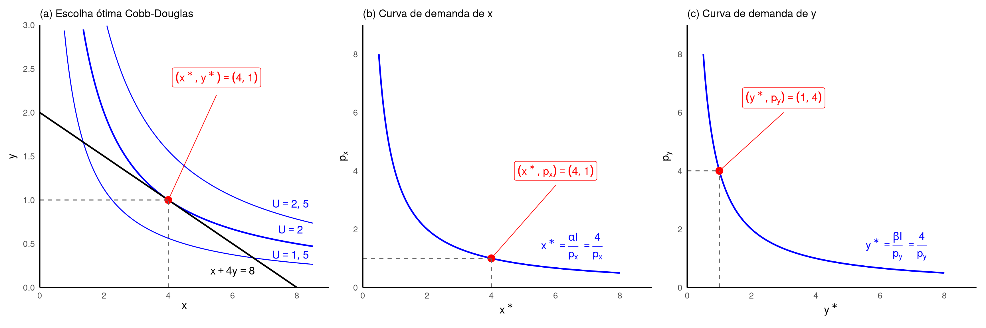
# Parâmetros
alpha <- 0.5
beta <- 1 - alpha
px <- 1
py <- 4
I_renda <- 8

# Demandas ótimas
x_star <- alpha * I_renda / px  # 4
y_star <- beta * I_renda / py   # 1
U_star <- x_star^alpha * y_star^beta  # 2

# --- Painel (a): Escolha ótima Cobb-Douglas ---
p1 <- ggplot() +
  # Curvas de indiferença: y = k^2 / x (para U = k, com alpha = beta = 0.5)
  geom_function(
    fun = \(x) 1.5^2 / x, xlim = c(0.3, 8.5), n = 300,
    color = "blue", linewidth = 0.6
  ) +
  geom_function(
    fun = \(x) 2^2 / x, xlim = c(0.5, 8.5), n = 300,
    color = "blue", linewidth = 1
  ) +
  geom_function(
    fun = \(x) 2.5^2 / x, xlim = c(0.8, 8.5), n = 300,
    color = "blue", linewidth = 0.6
  ) +
  # Rótulos das CIs
  annotate("text", x = 7.8, y = 1.3^2 / 7.8 + 0.15,
           label = latex2exp::TeX(r"($U = 1{,}5$)"),
           size = 5, color = "blue") +
  annotate("text", x = 7.8, y = 2^2 / 7.8 + 0.15,
           label = latex2exp::TeX(r"($U = 2$)"),
           size = 5, color = "blue") +
  annotate("text", x = 7.8, y = 2.5^2 / 7.8 + 0.15,
           label = latex2exp::TeX(r"($U = 2{,}5$)"),
           size = 5, color = "blue") +
  # Reta orçamentária
  geom_segment(
    aes(x = 0, y = I_renda / py, xend = I_renda / px, yend = 0),
    color = "black", linewidth = 1
  ) +
  # Rótulo da reta orçamentária
  annotate("text", x = 6, y = 0.18,
           label = latex2exp::TeX(r"($x + 4y = 8$)"),
           size = 5, color = "black") +
  # Ponto ótimo
  geom_point(aes(x = x_star, y = y_star), size = 4, color = "red") +
  # Projeções tracejadas
  geom_segment(
    aes(x = x_star, y = 0, xend = x_star, yend = y_star),
    linetype = "dashed", color = "gray40"
  ) +
  geom_segment(
    aes(x = 0, y = y_star, xend = x_star, yend = y_star),
    linetype = "dashed", color = "gray40"
  ) +
  # Linha conectando o ponto ao rótulo
  geom_segment(
    aes(x = x_star, y = y_star, xend = 5.5, yend = 2.2),
    color = "red", linewidth = 0.4
  ) +
  # Rótulo do ponto ótimo
  annotate("label", x = 5.5, y = 2.4,
           label = latex2exp::TeX(r"($(x^*, y^*) = (4, 1)$)"),
           size = 5, color = "red",
           fill = "white", label.size = 0.3) +
  scale_x_continuous(
    expand = c(0, 0),
    limits = c(0, 9),
    breaks = seq(0, 8, 2)
  ) +
  scale_y_continuous(
    expand = c(0, 0),
    limits = c(0, 3),
    breaks = seq(0, 3, 0.5)
  ) +
  labs(
    x = latex2exp::TeX(r"($x$)"),
    y = latex2exp::TeX(r"($y$)"),
    title = "(a) Escolha ótima Cobb-Douglas"
  ) +
  theme_minimal(base_size = 14) +
  theme(
    axis.line  = element_line(color = "black", linewidth = 0.8),
    panel.grid = element_blank(),
    axis.title = element_text(size = 14),
    plot.title = element_text(size = 14)
  )

# --- Painel (b): Curva de demanda de x ---
# Demanda inversa: p_x = alpha * I / x = 4 / x
p2 <- ggplot() +
  geom_function(
    fun = \(x) alpha * I_renda / x, xlim = c(0.5, 8), n = 300,
    color = "blue", linewidth = 1
  ) +
  # Rótulo da curva
  annotate("text", x = 6.5, y = alpha * I_renda / 6.5 + 0.8,
           label = latex2exp::TeX(r"($x^* = \frac{\alpha I}{p_x} = \frac{4}{p_x}$)"),
           size = 5, color = "blue") +
  # Ponto de referência (x* = 4, px = 1)
  geom_point(aes(x = x_star, y = px), size = 4, color = "red") +
  # Projeções tracejadas
  geom_segment(
    aes(x = x_star, y = 0, xend = x_star, yend = px),
    linetype = "dashed", color = "gray40"
  ) +
  geom_segment(
    aes(x = 0, y = px, xend = x_star, yend = px),
    linetype = "dashed", color = "gray40"
  ) +
  # Linha conectando o ponto ao rótulo
  geom_segment(
    aes(x = x_star, y = px, xend = 6, yend = 3.5),
    color = "red", linewidth = 0.4
  ) +
  # Rótulo do ponto
  annotate("label", x = 6, y = 4,
           label = latex2exp::TeX(r"($(x^*, p_x) = (4, 1)$)"),
           size = 5, color = "red",
           fill = "white", label.size = 0.3) +
  scale_x_continuous(
    expand = c(0, 0),
    limits = c(0, 9),
    breaks = seq(0, 8, 2)
  ) +
  scale_y_continuous(
    expand = c(0, 0),
    limits = c(0, 9),
    breaks = seq(0, 8, 2)
  ) +
  labs(
    x = latex2exp::TeX(r"($x^*$)"),
    y = latex2exp::TeX(r"($p_x$)"),
    title = "(b) Curva de demanda de x"
  ) +
  theme_minimal(base_size = 14) +
  theme(
    axis.line  = element_line(color = "black", linewidth = 0.8),
    panel.grid = element_blank(),
    axis.title = element_text(size = 14),
    plot.title = element_text(size = 14)
  )

# --- Painel (c): Curva de demanda de y ---
p3 <- ggplot() +
  geom_function(
    fun = \(y) beta * I_renda / y, xlim = c(0.5, 8), n = 300,
    color = "blue", linewidth = 1
  ) +
  # Rótulo da curva
  annotate("text", x = 6.5, y = beta * I_renda / 6.5 + 0.8,
           label = latex2exp::TeX(r"($y^* = \frac{\beta I}{p_y} = \frac{4}{p_y}$)"),
           size = 5, color = "blue") +
  # Ponto de referência (y* = 1, py = 4)
  geom_point(aes(x = y_star, y = py), size = 4, color = "red") +
  # Projeções tracejadas
  geom_segment(
    aes(x = y_star, y = 0, xend = y_star, yend = py),
    linetype = "dashed", color = "gray40"
  ) +
  geom_segment(
    aes(x = 0, y = py, xend = y_star, yend = py),
    linetype = "dashed", color = "gray40"
  ) +
  # Linha conectando o ponto ao rótulo
  geom_segment(
    aes(x = y_star, y = py, xend = 3, yend = 6),
    color = "red", linewidth = 0.4
  ) +
  # Rótulo do ponto
  annotate("label", x = 3, y = 6.5,
           label = latex2exp::TeX(r"($(y^*, p_y) = (1, 4)$)"),
           size = 5, color = "red",
           fill = "white", label.size = 0.3) +
  scale_x_continuous(
    expand = c(0, 0),
    limits = c(0, 9),
    breaks = seq(0, 8, 2)
  ) +
  scale_y_continuous(
    expand = c(0, 0),
    limits = c(0, 9),
    breaks = seq(0, 8, 2)
  ) +
  labs(
    x = latex2exp::TeX(r"($y^*$)"),
    y = latex2exp::TeX(r"($p_y$)"),
    title = "(c) Curva de demanda de y"
  ) +
  theme_minimal(base_size = 14) +
  theme(
    axis.line  = element_line(color = "black", linewidth = 0.8),
    panel.grid = element_blank(),
    axis.title = element_text(size = 14),
    plot.title = element_text(size = 14)
  )

# Combinar painéis
p1 + p2 + p3

Interpretação

As funções de demanda Cobb-Douglas possuem uma estrutura notavelmente simples: a demanda depende apenas do preço próprio e da renda, não dos preços dos outros bens.
As frações da renda são constantes determinadas pelos parâmetros de preferência ($\alpha$, $\beta$), não pelas condições de mercado.
A curva de demanda $x^*(p_x) = \alpha I/p_x$ é uma hipérbole retangular com elasticidade-preço unitária: um aumento de 1% no preço causa exatamente 1% de redução na quantidade demandada.
Essas propriedades tornam a Cobb-Douglas analiticamente conveniente, porém empiricamente restritiva.
A função CES (Note 4.6) relaxa a restrição de frações da renda constantes.

Nota 4.6: Funções de demanda CES

Símbolo	Significado
$U(x,y) = (x^\delta + y^\delta)^{1/\delta}$	função de utilidade CES (elasticidade de substituição constante)
$\delta$	parâmetro de substituição ($\delta \leq 1$, $\delta \neq 0$)
$\sigma = 1/(1 - \delta)$	elasticidade de substituição
$\delta \to 0$ ($\sigma = 1$)	caso limite: Cobb-Douglas
$\delta = 0{,}5$ ($\sigma = 2$)	alta substituibilidade
$\delta = -1$ ($\sigma = 0{,}5$)	baixa substituibilidade
$\delta \to -\infty$ ($\sigma \to 0$)	proporções fixas (complementos perfeitos)

Desenvolvimento teórico

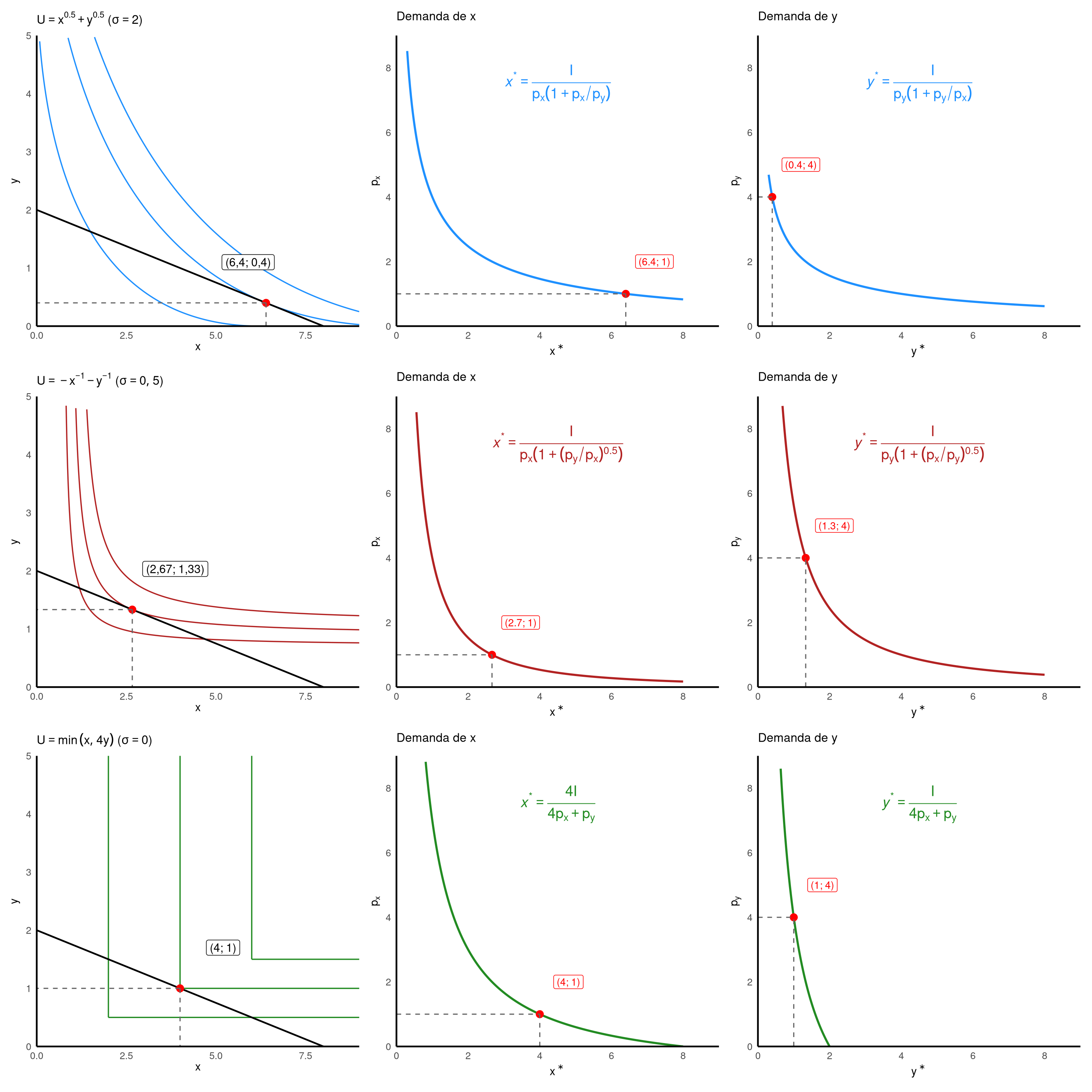
A função CES (Constant Elasticity of Substitution) engloba múltiplas estruturas de preferências dependendo do parâmetro $\delta$. Derivamos as funções de demanda para 3 casos a fim de mostrar como a elasticidade de substituição afeta o comportamento do consumidor.

Caso 1: $\delta = 0{,}5$ ($\sigma = 2$, alta substituibilidade)

$U(x,y) = x^{0{,}5} + y^{0{,}5}$

Note a diferença em relação à Cobb-Douglas: aqui os termos são somados, não multiplicados. Isso permite que o consumidor substitua mais livremente entre os bens.

Passo 1: Montar o Lagrangiano.

\[\mathscr{L} = x^{0{,}5} + y^{0{,}5} + \lambda(I - p_x x - p_y y)\]

Passo 2: Condições de primeira ordem.

\[\begin{aligned} \frac{\partial \mathscr{L}}{\partial x} &= 0{,}5\, x^{-0{,}5} - \lambda p_x = 0 & & \text{(CPO 1)} \\[6pt] \frac{\partial \mathscr{L}}{\partial y} &= 0{,}5\, y^{-0{,}5} - \lambda p_y = 0 & & \text{(CPO 2)} \\[6pt] \frac{\partial \mathscr{L}}{\partial \lambda} &= I - p_x x - p_y y = 0 & & \text{(CPO 3): restrição orçamentária} \end{aligned}\]

Passo 3: Dividir CPO 1 pela CPO 2 para eliminar $\lambda$. \[\begin{aligned} \frac{0{,}5\, x^{-0{,}5}}{0{,}5\, y^{-0{,}5}} &= \frac{\lambda p_x}{\lambda p_y} & & \text{dividindo membro a membro} \\[6pt] \frac{y^{0{,}5}}{x^{0{,}5}} &= \frac{p_x}{p_y} & & \text{cancelando } 0{,}5 \text{ e } \lambda \text{; invertendo } y^{-0{,}5} = 1/y^{0{,}5} \\[6pt] \left(\frac{y}{x}\right)^{0{,}5} &= \frac{p_x}{p_y} & & \text{reescrevendo o lado esquerdo} \\[6pt] \frac{y}{x} &= \left(\frac{p_x}{p_y}\right)^2 & & \text{elevando ambos os lados ao quadrado} \\[6pt] y &= x \left(\frac{p_x}{p_y}\right)^2 & & \text{isolando } y \end{aligned}\]

Passo 4: Substituir na restrição orçamentária.

\[\begin{aligned} p_x x + p_y \cdot x \left(\frac{p_x}{p_y}\right)^2 &= I & & \text{substituindo } y \\[6pt] p_x x + x \cdot \frac{p_x^2}{p_y} &= I & & \text{simplificando } p_y \text{ com } p_y^2 \\[6pt] p_x x \left(1 + \frac{p_x}{p_y}\right) &= I & & \text{colocando } p_x x \text{ em evidência} \\[6pt] x^* &= \frac{I}{p_x\!\left[1 + (p_x/p_y)\right]} \end{aligned}\]

\[\boxed{x^* = \frac{I}{p_x\!\left[1 + (p_x/p_y)\right]}}\]

Por simetria da função utilidade (trocando $x \leftrightarrow y$ e $p_x \leftrightarrow p_y$):

\[\boxed{y^* = \frac{I}{p_y\!\left[1 + (p_y/p_x)\right]}}\]

Passo 5: Fração da renda.

\[\begin{aligned} s_x &= \frac{p_x x^*}{I} & & \text{definição} \\[6pt] &= \frac{p_x}{I} \cdot \frac{I}{p_x[1 + (p_x/p_y)]} & & \text{substituindo } x^* \\[6pt] &= \frac{1}{1 + (p_x/p_y)} & & p_x \text{ e } I \text{ se cancelam} \end{aligned}\]

A participação diminui conforme $p_x/p_y$ aumenta — diferente da CD, onde a fração é constante. Quanto maior o preço relativo de $x$, menor a parcela gasta em $x$. A demanda é mais sensível a preços do que a Cobb-Douglas (expoente implícito sobre o preço próprio: $-2$ vs. $-1$ para CD).

Caso 2: $\delta = -1$ ($\sigma = 0{,}5$, baixa substituibilidade)

$U(x,y) = -x^{-1} - y^{-1}$

Com $\sigma = 0{,}5 < 1$, os bens são menos substituíveis que na Cobb-Douglas. O consumidor resiste mais a trocar um bem pelo outro quando preços mudam.

Passo 1: Montar o Lagrangiano.

\[\mathscr{L} = -x^{-1} - y^{-1} + \lambda(I - p_x x - p_y y)\]

Passo 2: Condições de primeira ordem.

\[\begin{aligned} \frac{\partial \mathscr{L}}{\partial x} &= x^{-2} - \lambda p_x = 0 & & \text{(CPO 1): derivada de } -x^{-1} \text{ é } x^{-2} \\[6pt] \frac{\partial \mathscr{L}}{\partial y} &= y^{-2} - \lambda p_y = 0 & & \text{(CPO 2): derivada de } -y^{-1} \text{ é } y^{-2} \\[6pt] \frac{\partial \mathscr{L}}{\partial \lambda} &= I - p_x x - p_y y = 0 & & \text{(CPO 3): restrição orçamentária} \end{aligned}\]

Passo 3: Dividir CPO 1 pela CPO 2 para eliminar $\lambda$. \[\begin{aligned} \frac{x^{-2}}{y^{-2}} &= \frac{\lambda p_x}{\lambda p_y} & & \text{dividindo membro a membro} \\[6pt] \frac{y^{2}}{x^{2}} &= \frac{p_x}{p_y} & & \text{cancelando } \lambda \text{; invertendo } x^{-2} = 1/x^{2} \\[6pt] \left(\frac{y}{x}\right)^{2} &= \frac{p_x}{p_y} & & \text{reescrevendo o lado esquerdo} \\[6pt] \frac{y}{x} &= \left(\frac{p_x}{p_y}\right)^{0{,}5} & & \text{tirando a raiz quadrada} \\[6pt] y &= x \left(\frac{p_x}{p_y}\right)^{0{,}5} & & \text{isolando } y \end{aligned}\]

Passo 4: Substituir na restrição orçamentária.

\[\begin{aligned} p_x x + p_y \cdot x \left(\frac{p_x}{p_y}\right)^{0{,}5} &= I & & \text{substituindo } y \\[6pt] p_x x + x \cdot p_y^{0{,}5} \cdot p_x^{0{,}5} &= I & & p_y \cdot (p_x/p_y)^{0{,}5} = p_y^{0{,}5}\, p_x^{0{,}5} \\[6pt] p_x x \left(1 + \frac{p_y^{0{,}5}}{p_x^{0{,}5}}\right) &= I & & \text{colocando } p_x x \text{ em evidência} \\[6pt] p_x x \left[1 + \left(\frac{p_y}{p_x}\right)^{0{,}5}\right] &= I & & \text{reescrevendo a fração} \\[6pt] x^* &= \frac{I}{p_x\!\left[1 + (p_y/p_x)^{0{,}5}\right]} \end{aligned}\]

\[\boxed{x^* = \frac{I}{p_x\!\left[1 + (p_y/p_x)^{0{,}5}\right]}}\]

Por simetria:

\[\boxed{y^* = \frac{I}{p_y\!\left[1 + (p_x/p_y)^{0{,}5}\right]}}\]

Passo 5: Fração da renda.

\[\begin{aligned} s_x &= \frac{p_x x^*}{I} & & \text{definição} \\[6pt] &= \frac{p_x}{I} \cdot \frac{I}{p_x[1 + (p_y/p_x)^{0{,}5}]} & & \text{substituindo } x^* \\[6pt] &= \frac{1}{1 + (p_y/p_x)^{0{,}5}} & & p_x \text{ e } I \text{ se cancelam} \end{aligned}\]

A participação aumenta conforme $p_x$ sobe — o oposto do Caso 1. O consumidor reduz a quantidade de $x$ de forma tão modesta que o gasto total em $x$ sobe. A demanda é menos sensível a preços que a Cobb-Douglas (expoente implícito: $-0{,}5$ vs. $-1$ para CD).

Caso 3: $\delta \to -\infty$ ($\sigma \to 0$, proporções fixas)

$U(x,y) = \min(x, 4y)$

Com $\sigma = 0$, não há substituição entre os bens — são complementos perfeitos. O consumidor sempre consome na proporção fixa $x = 4y$, independentemente dos preços. Não é possível usar cálculo (a função não é diferenciável no vértice).

Note que $\delta \to -\infty$ é um caso limite, não um valor assumido: a fórmula CES $(x^\delta + y^\delta)^{1/\delta}$ permanece válida para qualquer $\delta < 0$, e converge para $\min(x, y)$ quando $\delta \to -\infty$. O mesmo ocorre com $\delta \to 0$ (converge para Cobb-Douglas).

Passo 1: A utilidade é maximizada no vértice $x = 4y$.

Passo 2: Substituir na restrição orçamentária. \[\begin{aligned} I &= p_x (4y) + p_y y & & \text{substituindo } x = 4y \\[6pt] I &= (4 p_x + p_y)\, y & & \text{colocando } y \text{ em evidência} \\[6pt] y^* &= \frac{I}{4 p_x + p_y} & & \text{isolando } y \end{aligned}\]

\[\boxed{y^* = \frac{I}{4 p_x + p_y}}\]

Para $x^*$:

\[\begin{aligned} x^* &= 4 y^* = \frac{4I}{4 p_x + p_y} & & \text{usando } x = 4y \end{aligned}\]

\[\boxed{x^* = \frac{4I}{4 p_x + p_y}}\]

Passo 3: Fração da renda.

\[\begin{aligned} s_x &= \frac{p_x x^*}{I} & & \text{definição} \\[6pt] &= \frac{p_x}{I} \cdot \frac{4I}{4 p_x + p_y} & & \text{substituindo } x^* \\[6pt] &= \frac{4 p_x}{4 p_x + p_y} & & I \text{ se cancela} \end{aligned}\]

A fração da renda aumenta monotonicamente com $p_x$. Como não há substituição, um aumento de $p_x$ não altera a proporção $x/y = 4$ — apenas reduz ambas as quantidades Nicholson e Snyder (2012).

Exercício resolvido

Compare os 3 casos com $p_x = 1$, $p_y = 4$, $I = 8$ (mesmos parâmetros do Note 4.5, onde a CD deu $x^* = 4$, $y^* = 1$, $s_x = 0{,}50$).

Caso 1 ($\delta = 0{,}5$, $\sigma = 2$, alta substituibilidade):

\[\begin{aligned} x^* &= \frac{8}{1 \times [1 + (1/4)]} = \frac{8}{1{,}25} = 6{,}4 \\[6pt] y^* &= \frac{8}{4 \times [1 + (4/1)]} = \frac{8}{20} = 0{,}4 \\[6pt] s_x &= \frac{1}{1 + 0{,}25} = 0{,}80 \end{aligned}\]

O consumidor concentra 80% da renda em $x$ (o bem barato). Como $\sigma = 2 > 1$, ele substitui fortemente em direção ao bem mais barato. Comparando com a CD ($s_x = 0{,}50$): a alta substituibilidade faz o consumidor “fugir” do bem caro.

Caso 2 ($\delta = -1$, $\sigma = 0{,}5$, baixa substituibilidade):

\[\begin{aligned} x^* &= \frac{8}{1 \times [1 + (4)^{0{,}5}]} = \frac{8}{1 + 2} = \frac{8}{3} \approx 2{,}67 \\[6pt] y^* &= \frac{8}{4 \times [1 + (0{,}25)^{0{,}5}]} = \frac{8}{4 \times 1{,}5} = \frac{8}{6} \approx 1{,}33 \\[6pt] s_x &= \frac{1}{1 + 2} = \frac{1}{3} \approx 0{,}33 \end{aligned}\]

O consumidor gasta apenas 33% em $x$. Apesar de $x$ ser mais barato, a baixa substituibilidade impede uma forte migração: ele “precisa” de $y$ e aceita pagar caro. Comparando com a CD ($s_x = 0{,}50$): a baixa $\sigma$ protege o gasto no bem caro.

Caso 3 ($\delta \to -\infty$, $\sigma = 0$, complementos perfeitos):

\[\begin{aligned} x^* &= \frac{4 \times 8}{4 \times 1 + 4} = \frac{32}{8} = 4 \\[6pt] y^* &= \frac{8}{4 \times 1 + 4} = \frac{8}{8} = 1 \\[6pt] s_x &= \frac{4 \times 1}{4 \times 1 + 4} = \frac{4}{8} = 0{,}50 \end{aligned}\]

Proporção fixa: $x/y = 4$ sempre. Os preços não afetam a composição da cesta, apenas o nível de consumo. Coincidência: neste exemplo, $s_x = 0{,}50$ — igual à CD — mas por razões completamente diferentes (proporção fixa, não frações constantes).

Caso	$U(x,y)$	$\sigma$	$x^*$	$y^*$	$s_x$	Comportamento
1	$x^{0{,}5} + y^{0{,}5}$	$2$	$6{,}4$	$0{,}4$	$0{,}80$	Concentra no bem barato
CD	$x^{0{,}5} y^{0{,}5}$	$1$	$4$	$1$	$0{,}50$	Fração constante (referência)
2	$-x^{-1} - y^{-1}$	$0{,}5$	$2{,}67$	$1{,}33$	$0{,}33$	Protege o bem caro
3	$\min(x, 4y)$	$0$	$4$	$1$	$0{,}50$	Proporção fixa

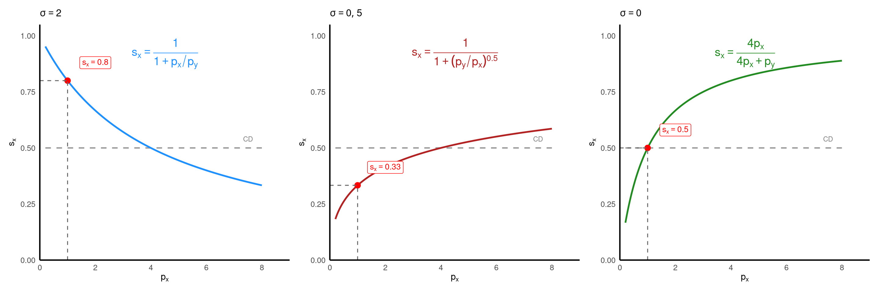
A tabela revela o papel central de $\sigma$: à medida que a elasticidade de substituição diminui, o consumidor migra menos em direção ao bem barato. No extremo ($\sigma = 0$), preços não afetam a composição da cesta.

Implementação em R

Código

suppressPackageStartupMessages({
  library(ggplot2)
  library(latex2exp)
  library(patchwork)
})

# Parâmetros comuns
px <- 1; py <- 4; I_renda <- 8
x_seq <- seq(0.01, 9, length.out = 500)

# Cores consistentes para os 3 casos
cor1 <- "dodgerblue"    # sigma = 2
cor2 <- "firebrick"     # sigma = 0.5
cor3 <- "forestgreen"   # sigma = 0 (Leontief)

# Restrição orçamentária
bl_x0 <- 0; bl_y0 <- I_renda / py
bl_x1 <- I_renda / px; bl_y1 <- 0

tema <- theme_minimal(base_size = 12) +
  theme(
    axis.line  = element_line(color = "black", linewidth = 0.8),
    panel.grid = element_blank(),
    axis.title = element_text(size = 11),
    plot.title = element_text(size = 12)
  )

# Função auxiliar: gráfico de demanda (x* horizontal, preço vertical)
graf_demanda <- function(dem_fun, cor, titulo, eixo_q, eixo_p, q_ref, p_ref,
                         label_eq = NULL) {
  p <- ggplot() +
    geom_function(
      fun = dem_fun, xlim = c(0.3, 8), n = 300,
      color = cor, linewidth = 1
    ) +
    geom_point(aes(x = q_ref, y = p_ref), size = 3, color = "red") +
    geom_segment(
      aes(x = q_ref, y = 0, xend = q_ref, yend = p_ref),
      linetype = "dashed", color = "gray40"
    ) +
    geom_segment(
      aes(x = 0, y = p_ref, xend = q_ref, yend = p_ref),
      linetype = "dashed", color = "gray40"
    ) +
    annotate("label", x = q_ref + 0.8, y = p_ref + 1,
             label = paste0("(", round(q_ref, 1), "; ", round(p_ref, 0), ")"),
             size = 3.5, color = "red", fill = "white", label.size = 0.2) +
    scale_x_continuous(expand = c(0, 0), limits = c(0, 9), breaks = seq(0, 8, 2)) +
    scale_y_continuous(expand = c(0, 0), limits = c(0, 9), breaks = seq(0, 8, 2)) +
    labs(x = eixo_q, y = eixo_p, title = titulo) +
    tema
  if (!is.null(label_eq)) {
    p <- p + annotate("text", x = 4.5, y = 7.5, label = label_eq,
                      size = 5, color = cor, parse = TRUE)
  }
  p
}

# ============================================================
# LINHA 1: Caso 1 — U = x^0.5 + y^0.5 (sigma = 2)
# ============================================================
x1_star <- 6.4; y1_star <- 0.4

k_vals_a <- c(2.5, sqrt(x1_star) + sqrt(y1_star), 3.5)
df_ic_a <- do.call(rbind, lapply(seq_along(k_vals_a), function(i) {
  k <- k_vals_a[i]
  x <- x_seq[x_seq <= k^2]
  y <- (k - sqrt(x))^2
  data.frame(x = x, y = y, curva = factor(i))
}))

p1_u <- ggplot() +
  geom_line(data = df_ic_a, aes(x = x, y = y, group = curva),
            color = cor1, linewidth = 0.6) +
  geom_segment(aes(x = bl_x0, y = bl_y0, xend = bl_x1, yend = bl_y1),
               colour = "black", linewidth = 0.8) +
  geom_point(aes(x = x1_star, y = y1_star), size = 3, colour = "red") +
  geom_segment(aes(x = x1_star, y = y1_star, xend = x1_star, yend = 0),
               linetype = "dashed", colour = "grey40") +
  geom_segment(aes(x = x1_star, y = y1_star, xend = 0, yend = y1_star),
               linetype = "dashed", colour = "grey40") +
  annotate("label", x = x1_star - 0.5, y = y1_star + 0.7,
           label = "(6,4; 0,4)", size = 4, fill = "white", label.size = 0.2) +
  scale_x_continuous(limits = c(0, 9), expand = c(0, 0)) +
  scale_y_continuous(limits = c(0, 5), expand = c(0, 0)) +
  labs(x = TeX(r"($x$)"), y = TeX(r"($y$)"),
       title = TeX(r"($U = x^{0.5} + y^{0.5}$ ($\sigma = 2$))")) +
  tema

# Demanda de x: x*(px) = I / (px * (1 + px/py)), py = 4 fixo
# Demanda inversa: para plotar px no eixo y, dado x no eixo x
dem_x1 <- function(x) I_renda / (x * (1 + x * py / I_renda))
# Mais simples: usar a demanda inversa numericamente
dem_x1_inv <- function(q) {
  # x* = I / (px * (1 + px/py)) => resolver para px dado q
  # Usar a função direta para plotar: px -> x*(px)
  sapply(q, function(qi) {
    tryCatch(uniroot(function(p) I_renda / (p * (1 + p / py)) - qi,
                     c(0.01, 100))$root, error = function(e) NA)
  })
}
# Alternativa direta: plotar px vs x*(px)
dem_x1_dir <- function(px) I_renda / (px * (1 + px / py))

p1_dx <- graf_demanda(
  \(q) sapply(q, function(qi)
    tryCatch(uniroot(\(p) I_renda / (p * (1 + p / py)) - qi,
             c(0.001, 200))$root, error = \(e) NA)),
  cor1, "Demanda de x",
  TeX(r"($x^*$)"), TeX(r"($p_x$)"), x1_star, px,
  "italic(x)^'*' == frac(I, p[x]*(1 + p[x]/p[y]))")

# Demanda de y: y*(py) = I / (py * (1 + py/px)), px = 1 fixo
p1_dy <- graf_demanda(
  \(q) sapply(q, function(qi)
    tryCatch(uniroot(\(p) I_renda / (p * (1 + p / px)) - qi,
             c(0.001, 200))$root, error = \(e) NA)),
  cor1, "Demanda de y",
  TeX(r"($y^*$)"), TeX(r"($p_y$)"), y1_star, py,
  "italic(y)^'*' == frac(I, p[y]*(1 + p[y]/p[x]))")

# ============================================================
# LINHA 2: Caso 2 — U = -x^{-1} - y^{-1} (sigma = 0.5)
# ============================================================
x2_star <- 8 / 3; y2_star <- 4 / 3

k_opt_b <- -1 / x2_star - 1 / y2_star
k_vals_b <- c(k_opt_b - 0.3, k_opt_b, k_opt_b + 0.2)
df_ic_b <- do.call(rbind, lapply(seq_along(k_vals_b), function(i) {
  k <- k_vals_b[i]
  x <- x_seq; denom <- k + 1 / x; y <- -1 / denom
  valid <- y > 0 & y < 5
  data.frame(x = x[valid], y = y[valid], curva = factor(i))
}))

p2_u <- ggplot() +
  geom_line(data = df_ic_b, aes(x = x, y = y, group = curva),
            color = cor2, linewidth = 0.6) +
  geom_segment(aes(x = bl_x0, y = bl_y0, xend = bl_x1, yend = bl_y1),
               colour = "black", linewidth = 0.8) +
  geom_point(aes(x = x2_star, y = y2_star), size = 3, colour = "red") +
  geom_segment(aes(x = x2_star, y = y2_star, xend = x2_star, yend = 0),
               linetype = "dashed", colour = "grey40") +
  geom_segment(aes(x = x2_star, y = y2_star, xend = 0, yend = y2_star),
               linetype = "dashed", colour = "grey40") +
  annotate("label", x = x2_star + 1.2, y = y2_star + 0.7,
           label = "(2,67; 1,33)", size = 4, fill = "white", label.size = 0.2) +
  scale_x_continuous(limits = c(0, 9), expand = c(0, 0)) +
  scale_y_continuous(limits = c(0, 5), expand = c(0, 0)) +
  labs(x = TeX(r"($x$)"), y = TeX(r"($y$)"),
       title = TeX(r"($U = -x^{-1} - y^{-1}$ ($\sigma = 0{,}5$))")) +
  tema

# Demanda de x: x*(px) = I / (px * (1 + (py/px)^0.5))
p2_dx <- graf_demanda(
  \(q) sapply(q, function(qi)
    tryCatch(uniroot(\(p) I_renda / (p * (1 + (py / p)^0.5)) - qi,
             c(0.001, 200))$root, error = \(e) NA)),
  cor2, "Demanda de x",
  TeX(r"($x^*$)"), TeX(r"($p_x$)"), x2_star, px,
  "italic(x)^'*' == frac(I, p[x]*(1 + (p[y]/p[x])^0.5))")

# Demanda de y: y*(py) = I / (py * (1 + (px/py)^0.5))
p2_dy <- graf_demanda(
  \(q) sapply(q, function(qi)
    tryCatch(uniroot(\(p) I_renda / (p * (1 + (px / p)^0.5)) - qi,
             c(0.001, 200))$root, error = \(e) NA)),
  cor2, "Demanda de y",
  TeX(r"($y^*$)"), TeX(r"($p_y$)"), y2_star, py,
  "italic(y)^'*' == frac(I, p[y]*(1 + (p[x]/p[y])^0.5))")

# ============================================================
# LINHA 3: Caso 3 — U = min(x, 4y) (sigma = 0, Leontief)
# ============================================================
x3_star <- 4; y3_star <- 1

k_vals_c <- c(2, 4, 6)
df_seg_c <- do.call(rbind, lapply(k_vals_c, function(k) {
  rbind(
    data.frame(x = k, y = k / 4, xend = 9, yend = k / 4, k = factor(k)),
    data.frame(x = k, y = k / 4, xend = k, yend = 5, k = factor(k))
  )
}))

p3_u <- ggplot() +
  geom_segment(data = df_seg_c,
               aes(x = x, y = y, xend = xend, yend = yend, group = k),
               color = cor3, linewidth = 0.6) +
  geom_segment(aes(x = bl_x0, y = bl_y0, xend = bl_x1, yend = bl_y1),
               colour = "black", linewidth = 0.8) +
  geom_point(aes(x = x3_star, y = y3_star), size = 3, colour = "red") +
  geom_segment(aes(x = x3_star, y = y3_star, xend = x3_star, yend = 0),
               linetype = "dashed", colour = "grey40") +
  geom_segment(aes(x = x3_star, y = y3_star, xend = 0, yend = y3_star),
               linetype = "dashed", colour = "grey40") +
  annotate("label", x = x3_star + 1.2, y = y3_star + 0.7,
           label = "(4; 1)", size = 4, fill = "white", label.size = 0.2) +
  scale_x_continuous(limits = c(0, 9), expand = c(0, 0)) +
  scale_y_continuous(limits = c(0, 5), expand = c(0, 0)) +
  labs(x = TeX(r"($x$)"), y = TeX(r"($y$)"),
       title = TeX(r"($U = \min(x, 4y)$ ($\sigma = 0$))")) +
  tema

# Demanda de x: x*(px) = 4I / (4px + py)
p3_dx <- graf_demanda(
  \(q) (4 * I_renda / q - py) / 4,
  cor3, "Demanda de x",
  TeX(r"($x^*$)"), TeX(r"($p_x$)"), x3_star, px,
  "italic(x)^'*' == frac(4*I, 4*p[x] + p[y])")

# Demanda de y: y*(py) = I / (4px + py)
p3_dy <- graf_demanda(
  \(q) I_renda / q - 4 * px,
  cor3, "Demanda de y",
  TeX(r"($y^*$)"), TeX(r"($p_y$)"), y3_star, py,
  "italic(y)^'*' == frac(I, 4*p[x] + p[y])")

# Combinar: 3 linhas × 3 colunas
(p1_u | p1_dx | p1_dy) /
(p2_u | p2_dx | p2_dy) /
(p3_u | p3_dx | p3_dy)

Código

suppressPackageStartupMessages({
  library(ggplot2)
  library(latex2exp)
  library(patchwork)
})

px <- 1; py <- 4; I_renda <- 8

# Cores consistentes
cor1 <- "dodgerblue"    # sigma = 2
cor2 <- "firebrick"     # sigma = 0.5
cor3 <- "forestgreen"   # sigma = 0

tema <- theme_minimal(base_size = 12) +
  theme(
    axis.line  = element_line(color = "black", linewidth = 0.8),
    panel.grid = element_blank(),
    axis.title = element_text(size = 11),
    plot.title = element_text(size = 12)
  )

# CD como referência (linha tracejada cinza em todos os painéis)
sx_cd <- function(px) rep(0.5, length(px))

# Função auxiliar: mini gráfico de fração da renda
mini_share <- function(sx_fun, cor, titulo, sx_ref, label_eq) {
  ggplot() +
    # CD como referência
    geom_function(
      fun = sx_cd, xlim = c(0.2, 8), n = 300,
      color = "gray60", linewidth = 0.8, linetype = "dashed"
    ) +
    annotate("text", x = 7.5, y = 0.54, label = "CD",
             size = 3, color = "gray50") +
    # Curva do caso
    geom_function(
      fun = sx_fun, xlim = c(0.2, 8), n = 300,
      color = cor, linewidth = 1
    ) +
    # Ponto de referência em px = 1
    geom_point(aes(x = 1, y = sx_ref), size = 3, color = "red") +
    geom_segment(aes(x = 1, y = 0, xend = 1, yend = sx_ref),
                 linetype = "dashed", color = "gray40") +
    geom_segment(aes(x = 0, y = sx_ref, xend = 1, yend = sx_ref),
                 linetype = "dashed", color = "gray40") +
    annotate("label", x = 2, y = sx_ref + 0.08,
             label = paste0("s[x] == ", round(sx_ref, 2)),
             size = 3.5, color = "red", fill = "white",
             label.size = 0.2, parse = TRUE) +
    # Equação
    annotate("text", x = 4.5, y = 0.92, label = label_eq,
             size = 5, color = cor, parse = TRUE) +
    scale_x_continuous(expand = c(0, 0), limits = c(0, 9),
                       breaks = seq(0, 8, 2)) +
    scale_y_continuous(expand = c(0, 0), limits = c(0, 1.05),
                       breaks = seq(0, 1, 0.25)) +
    labs(x = TeX(r"($p_x$)"), y = TeX(r"($s_x$)"), title = titulo) +
    tema
}

p_s1 <- mini_share(
  \(px) 1 / (1 + px / py),
  cor1, TeX(r"($\sigma = 2$)"), 0.80,
  "s[x] == frac(1, 1 + p[x]/p[y])")

p_s2 <- mini_share(
  \(px) 1 / (1 + (py / px)^0.5),
  cor2, TeX(r"($\sigma = 0{,}5$)"), 1/3,
  "s[x] == frac(1, 1 + (p[y]/p[x])^0.5)")

p_s3 <- mini_share(
  \(px) 4 * px / (4 * px + py),
  cor3, TeX(r"($\sigma = 0$)"), 0.50,
  "s[x] == frac(4*p[x], 4*p[x] + p[y])")

p_s1 + p_s2 + p_s3

Interpretação

A família CES como espectro de substituibilidade. A função CES unifica, num único parâmetro $\sigma$, todo o espectro de comportamento do consumidor:

$\sigma$ (elasticidade de substituição)	Curvas de indiferença	Demanda	Fração da renda $s_x$ quando $p_x \uparrow$
$\sigma > 1$	Achatadas (quase retas)	Muito elástica	Cai — foge do bem caro
$\sigma = 1$ (CD)	Hipérboles	Elasticidade unitária	Constante — gasta fração fixa
$\sigma < 1$	Angulares (quase L)	Pouco elástica	Sobe — “preso” ao bem caro
$\sigma = 0$	L (ângulo reto)	Perfeitamente inelástica	Sobe — proporção fixa

Leitura dos gráficos. Os painéis de demanda tornam visível o papel de $\sigma$: a curva de $\sigma = 2$ é quase horizontal (pequenas variações de preço causam grandes variações de quantidade), enquanto a de $\sigma = 0$ é quase vertical (preço muda, quantidade mal se altera). Os painéis de fração da renda revelam a consequência: quando $\sigma > 1$, o consumidor substitui tanto que o gasto total no bem caro diminui; quando $\sigma < 1$, substitui tão pouco que o gasto total aumenta.

Por que $\sigma$ importa? Em política econômica, $\sigma$ determina quem absorve o impacto de um aumento de preço. Se energia e alimentos têm $\sigma$ baixo (pouca substituição), um aumento de preços atinge desproporcionalmente famílias de baixa renda — elas não conseguem substituir e gastam uma fração crescente do orçamento nesses bens. A Cobb-Douglas, com frações fixas, não captura esse efeito Nicholson e Snyder (2012).

Nota 4.7: Formalização avançada: o problema do consumidor

Este box apresenta a formulação rigorosa do problema do consumidor usada em livros de nível avançado (mestrado/doutorado), seguindo a notação e estrutura de Jehle e Reny (2011, cap. 1.3). O objetivo é mostrar como os mesmos conceitos dos callouts anteriores (restrição orçamentária, maximização via Lagrange, funções de demanda) são expressos com maior rigor matemático.

Notação

Símbolo	Significado
$X = \mathbb{R}^n_+$	conjunto de consumo
$\mathbf{x} = (x_1, \ldots, x_n) \in X$	cesta de consumo
$\succeq$	relação de preferência fraca
$u: \mathbb{R}^n_+ \to \mathbb{R}$	função de utilidade representando $\succeq$
$\mathbf{p} = (p_1, \ldots, p_n) \gg \mathbf{0}$	vetor de preços (todos estritamente positivos)
$y > 0$	renda nominal
$B = \{\mathbf{x} \in \mathbb{R}^n_+ : \mathbf{p} \cdot \mathbf{x} \leq y\}$	conjunto orçamentário (feasible set)
$\mathbf{x}^* = \mathbf{x}(\mathbf{p}, y)$	demanda marshalliana (solução do problema)

Os quatro blocos do modelo

O Jehle e Reny (2011, Seção 1.1) identifica quatro blocos que compõem qualquer modelo de escolha do consumidor:

Conjunto de consumo ($X$): todas as cestas concebíveis. Assumimos $X = \mathbb{R}^n_+$.
Conjunto factível ($B \subset X$): as cestas que o consumidor pode efetivamente adquirir, dadas suas restrições econômicas.
Relação de preferência ($\succeq$): descreve os gostos do consumidor — sua capacidade de comparar e ordenar alternativas.
Hipótese comportamental: o consumidor busca a alternativa mais preferida dentro do conjunto factível.

No Nicholson, esses blocos aparecem de forma implícita: o conjunto de consumo é o quadrante positivo, o conjunto factível é o triângulo orçamentário, as preferências são representadas por curvas de indiferença, e a hipótese comportamental é “maximizar utilidade”. O Jehle torna cada bloco explícito e preciso.

O problema do consumidor em duas formulações

O Jehle e Reny (2011) apresenta o problema do consumidor em dois níveis de abstração.

Formulação primitiva (preferências). O consumidor busca a cesta mais preferida dentro do conjunto factível:

\[\mathbf{x}^* \in B \quad \text{tal que} \quad \mathbf{x}^* \succeq \mathbf{x} \quad \text{para todo } \mathbf{x} \in B\]

Lê-se: “$\mathbf{x}^*$ pertence ao conjunto orçamentário $B$ e é pelo menos tão boa quanto qualquer outra cesta factível”. Esta formulação é mais geral: não requer que as preferências sejam representáveis por uma função de utilidade. Basta que o consumidor consiga comparar cestas ($\succeq$ completa e transitiva).

Formulação via função de utilidade. Sob as hipóteses de completude, transitividade, continuidade, monotonicidade estrita e convexidade estrita (Hipótese 1.2, Jehle), as preferências podem ser representadas por uma função $u$ contínua, estritamente crescente e estritamente quase-côncava. Essas são as hipóteses que garantem curvas de indiferença “bem comportadas” (sem cruzamentos, sem regiões planas, convexas em relação à origem). O problema torna-se:

\[\max_{\mathbf{x} \in \mathbb{R}^n_+} \; u(\mathbf{x}) \quad \text{s.a.} \quad \mathbf{p} \cdot \mathbf{x} \leq y\]

Compare com o Nicholson: $\max U(x_1, \ldots, x_n)$ s.a. $p_1 x_1 + \cdots + p_n x_n \leq I$. A estrutura é idêntica — as diferenças são puramente notacionais:

Nicholson	Jehle	Observação
$I$	$y$	renda nominal
$p_1 x_1 + \cdots + p_n x_n$	$\mathbf{p} \cdot \mathbf{x}$	gasto total (produto interno)
$U(x_1, \ldots, x_n)$	$u(\mathbf{x})$	função de utilidade

O conjunto orçamentário

No Nicholson, a restrição orçamentária para dois bens é $p_x x + p_y y \leq I$, com representação gráfica como um triângulo no plano $(x, y)$. No Jehle, a notação vetorial generaliza para $n$ bens:

\[B = \{\mathbf{x} \in \mathbb{R}^n_+ : \mathbf{p} \cdot \mathbf{x} \leq y\}\]

onde $\mathbf{p} \cdot \mathbf{x} = \sum_{i=1}^n p_i x_i$ é o produto interno (gasto total). Geometricamente, $B$ é um simplex (generalização do triângulo para $n$ dimensões).

Propriedades de $B$ que o Jehle utiliza:

Não-vazio: $\mathbf{0} \in B$ (o consumidor sempre pode “não comprar nada”)
Fechado: a fronteira $\mathbf{p} \cdot \mathbf{x} = y$ pertence a $B$ (inclui a igualdade $\leq$)
Limitado: com $p_i > 0$ para todo $i$ e $y$ finito, nenhuma quantidade pode ser infinita
Convexo: se $\mathbf{x}^1 \in B$ e $\mathbf{x}^2 \in B$, qualquer combinação $t\mathbf{x}^1 + (1-t)\mathbf{x}^2$ com $t \in [0,1]$ também pertence a $B$

As três primeiras propriedades (não-vazio, fechado, limitado) implicam que $B$ é compacto — um conceito topológico fundamental que garante a existência de máximo.

Por monotonicidade estrita, a solução $\mathbf{x}^*$ satisfaz a restrição com igualdade ($\mathbf{p} \cdot \mathbf{x}^* = y$): o consumidor gasta toda a renda. Se sobrasse dinheiro, ele poderia comprar mais de algum bem e aumentar sua utilidade. Portanto, a solução está na fronteira de $B$, não no interior.

Existência e unicidade da solução

Um aspecto que o Nicholson não discute explicitamente é: por que podemos ter certeza de que a solução existe e é única? O Jehle responde com dois resultados matemáticos.

Existência (Teorema de Weierstrass). Uma função contínua definida sobre um conjunto compacto atinge seu máximo. Como $u$ é contínua e $B$ é compacto (não-vazio, fechado, limitado), existe pelo menos um $\mathbf{x}^* \in B$ que maximiza $u$.

Em termos intuitivos: se o consumidor tem um orçamento finito e seus gostos não apresentam “saltos” (continuidade), ele sempre pode encontrar uma melhor escolha. Não existe a possibilidade de “aproximar-se infinitamente do ótimo sem alcançá-lo”.

Unicidade. Como $u$ é estritamente quase-côncava e $B$ é convexo, o máximo é único. Estrita quase-concavidade significa que as curvas de indiferença são estritamente convexas (sem segmentos lineares). Se houvesse dois pontos ótimos distintos $\mathbf{x}^1$ e $\mathbf{x}^2$ com $u(\mathbf{x}^1) = u(\mathbf{x}^2) = u^*$, então a combinação $t\mathbf{x}^1 + (1-t)\mathbf{x}^2$ (que pertence a $B$ por convexidade) teria utilidade $u > u^*$ (por quase-concavidade estrita), contradizendo a otimalidade.

Conexão com o Nicholson: no Note 4.2, vimos que “a TMS decrescente garante um máximo verdadeiro” e que “curvas de indiferença convexas” são condição suficiente. O Jehle formaliza essa intuição:

\[\text{TMS decrescente} \iff u \text{ estritamente quase-côncava} \iff \text{máximo único}\]

Demanda marshalliana

A solução do problema depende dos parâmetros $\mathbf{p}$ e $y$. Isso define as funções de demanda marshalliana (ou ordinária):

\[x_i^* = x_i(\mathbf{p}, y), \qquad i = 1, \ldots, n\]

ou em notação vetorial: $\mathbf{x}^* = \mathbf{x}(\mathbf{p}, y)$.

O Jehle enfatiza um ponto sutil: estas funções são o resultado de um problema de otimização, não uma relação empírica observada diretamente. A curva de demanda que se observa no mercado é a projeção dessas funções quando variamos um preço ($p_i$) e mantemos os demais preços e a renda fixos.

No Nicholson, derivamos exemplos concretos dessas funções: $x^* = \alpha I / p_x$ (Cobb-Douglas) e as demandas CES. Cada uma é um caso particular de $\mathbf{x}(\mathbf{p}, y)$ para uma forma funcional específica de $u$.

Propriedades gerais das demandas marshalianas (válidas para qualquer $u$ bem-comportada):

Homogeneidade de grau zero: $\mathbf{x}(t\mathbf{p}, ty) = \mathbf{x}(\mathbf{p}, y)$ para todo $t > 0$. Dobrar todos os preços e a renda simultaneamente não altera as quantidades demandadas — apenas valores nominais mudam, o poder de compra real permanece o mesmo.
Lei de Walras: $\mathbf{p} \cdot \mathbf{x}(\mathbf{p}, y) = y$. O consumidor gasta toda a renda (consequência da monotonicidade).

Condições de Kuhn-Tucker

Quando $u$ é diferenciável, as condições necessárias para o ótimo são as condições de Kuhn-Tucker (KKT). O Lagrangiano é:

\[\mathscr{L}(\mathbf{x}, \lambda) = u(\mathbf{x}) + \lambda(y - \mathbf{p} \cdot \mathbf{x})\]

Para solução interior ($\mathbf{x}^* \gg \mathbf{0}$), as condições necessárias são:

\[\frac{\partial u(\mathbf{x}^*)}{\partial x_i} = \lambda p_i, \qquad i = 1, \ldots, n\]

\[\mathbf{p} \cdot \mathbf{x}^* = y\]

Compare com as CPOs do Note 4.4: $\partial U/\partial x_i = \lambda p_i$. São idênticas — apenas a notação muda ($u$ em vez de $U$, $y$ em vez de $I$).

A TMS como razão de preços. Dividindo a condição do bem $i$ pela do bem $j$:

\[\frac{\partial u / \partial x_i}{\partial u / \partial x_j} = \frac{p_i}{p_j} \qquad \Leftrightarrow \qquad MRS_{ij}(\mathbf{x}^*) = \frac{p_i}{p_j}\]

Essa é exatamente a condição $TMS = p_x/p_y$ do Nicholson, agora expressa para qualquer par de bens $i, j$.

Interpretação de $\lambda$. O multiplicador $\lambda$ mede a variação marginal da utilidade máxima quando a renda aumenta em uma unidade:

\[\lambda = \frac{\partial u^*}{\partial y}\]

onde $u^* = u(\mathbf{x}^*(\mathbf{p}, y))$ é a utilidade indireta. No Nicholson, chamamos isso de “utilidade marginal da renda”. No Jehle, $\lambda$ é o “valor-sombra” (shadow value) da restrição orçamentária — o preço implícito de relaxar a restrição em uma unidade monetária.

Para soluções de canto ($x_i^* = 0$ para algum $i$), as condições tornam-se:

\[\frac{\partial u(\mathbf{x}^*)}{\partial x_i} \leq \lambda p_i, \qquad x_i^* \geq 0, \qquad x_i^* \left(\frac{\partial u}{\partial x_i} - \lambda p_i\right) = 0\]

A última equação é a condição de folga complementar: ou $x_i > 0$ e a igualdade vale, ou $x_i = 0$ e a desigualdade pode ser estrita. No Note 4.4, interpretamos isso como “o consumidor não compra bens cujo preço excede sua disposição a pagar”.

Conexão com os callouts anteriores

Conceito (Nicholson / callouts)	Formalização avançada (Jehle)
Restrição orçamentária $p_x x + p_y y \leq I$	Conjunto orçamentário $B = \{\mathbf{x} : \mathbf{p} \cdot \mathbf{x} \leq y\}$
$\max U(x,y)$ s.a. restrição	$\max u(\mathbf{x})$ s.a. $\mathbf{p} \cdot \mathbf{x} \leq y$
TMS decrescente garante máximo	$u$ estritamente quase-côncava $\Rightarrow$ máximo único
CPOs: $\partial U/\partial x_i = \lambda p_i$	Condições de Kuhn-Tucker (idênticas)
$TMS = p_x/p_y$	$MRS_{ij} = p_i/p_j$ (razão das utilidades marginais = razão de preços)
Funções de demanda $x^*(p_x, p_y, I)$	Demanda marshalliana $\mathbf{x}(\mathbf{p}, y)$
$\lambda$ = utilidade marginal da renda	$\lambda$ = valor-sombra da restrição orçamentária

Referência principal: (Jehle e Reny, 2011, cap. 1.3). Para uma abordagem alternativa com ênfase em dualidade, ver (Mas-Colell, Whinston e Green, 1995, cap. 3.D–3.G).

Símbolo	Significado
\(I\)	renda nominal do consumidor
\(p_x\), \(p_y\)	preços dos bens \(x\) e \(y\)
\(p_x x + p_y y \leq I\)	restrição orçamentária
\(I/p_x\)	intercepto horizontal (gastar tudo em \(x\))
\(I/p_y\)	intercepto vertical (gastar tudo em \(y\))
\(-p_x/p_y\)	inclinação da reta orçamentária (custo de oportunidade)

Forma geral	Restrição orçamentária	Significado econômico
\(b\)	\(\dfrac{I}{p_y}\)	Intercepto vertical: quantidade máxima de \(y\) se gastar tudo em \(y\)
\(a\)	\(-\dfrac{p_x}{p_y}\)	Coeficiente angular: quantas unidades de \(y\) são sacrificadas por cada unidade adicional de \(x\)
\(1/a\)	\(-\dfrac{p_y}{p_x}\)	Coeficiente angular inverso: quantas unidades de \(x\) são sacrificadas por cada unidade adicional de \(y\)
\(-b/a\)	\(\dfrac{I}{p_x}\)	Intercepto horizontal: quantidade máxima de \(x\) se gastar tudo em \(x\)

Símbolo	Significado
\(\mathscr{L}\)	função Lagrangiana
\(\lambda\)	multiplicador de Lagrange
\(U_i = \partial U/\partial x_i\)	utilidade marginal do bem \(i\)
\(\partial \mathscr{L}/\partial x_i = 0\)	condição de primeira ordem (CPO) para o bem \(i\)
\(U_i/p_i = \lambda\)	utilidade marginal por real gasto deve ser igual para todos os bens

Símbolo	Significado
\(U(x,y) = x^\alpha y^\beta\)	função de utilidade Cobb-Douglas
\(\alpha + \beta = 1\)	normalização dos expoentes
\(x^* = \alpha I / p_x\)	demanda ótima de \(x\)
\(y^* = \beta I / p_y\)	demanda ótima de \(y\)
\(s_x = p_x x^* / I = \alpha\)	fração da renda gasta em \(x\)

Caso	\(U(x,y)\)	\(\sigma\)	\(x^*\)	\(y^*\)	\(s_x\)	Comportamento
1	\(x^{0{,}5} + y^{0{,}5}\)	\(2\)	\(6{,}4\)	\(0{,}4\)	\(0{,}80\)	Concentra no bem barato
CD	\(x^{0{,}5} y^{0{,}5}\)	\(1\)	\(4\)	\(1\)	\(0{,}50\)	Fração constante (referência)
2	\(-x^{-1} - y^{-1}\)	\(0{,}5\)	\(2{,}67\)	\(1{,}33\)	\(0{,}33\)	Protege o bem caro
3	\(\min(x, 4y)\)	\(0\)	\(4\)	\(1\)	\(0{,}50\)	Proporção fixa

Por onde começar?

Revisão: a equação da reta

Desenvolvimento Teórico

Exercício Resolvido

Implementação em R

Interpretação

Desenvolvimento Teórico

Exercício Resolvido

Implementação em R

Interpretação

Revisão: o método de Lagrange

Exemplo: ingressos de futebol e cinema

Passo 1: montar o Lagrangiano

Passo 2: condições de primeira ordem

Passo 3: resolver o sistema

Passo 4: verificações

Implementação em R

Interpretação

O problema

Montagem do Lagrangiano

Condições de primeira ordem (CPOs)

Implicações das CPOs

Interpretação do multiplicador \(\lambda\)

Soluções de canto (condições de Kuhn-Tucker)

Exercício resolvido

Interpretação

Desenvolvimento Teórico

Exercício Resolvido

Implementação em R

Interpretação

Desenvolvimento teórico

Caso 1: \(\delta = 0{,}5\) (\(\sigma = 2\), alta substituibilidade)

Caso 2: \(\delta = -1\) (\(\sigma = 0{,}5\), baixa substituibilidade)

Caso 3: \(\delta \to -\infty\) (\(\sigma \to 0\), proporções fixas)

Exercício resolvido

Implementação em R

Interpretação

Notação

Os quatro blocos do modelo

O problema do consumidor em duas formulações

O conjunto orçamentário

Existência e unicidade da solução

Demanda marshalliana

Condições de Kuhn-Tucker

Conexão com os callouts anteriores

Referências