Material de referência:Varian (2012) Capítulo 33 — Production.
Acesse o PDF na janela abaixo ↓.
Introdução
O equilíbrio geral com produção estende a análise de equilíbrio geral de trocas ao incorporar a produção de bens(Varian, 2012). Enquanto no modelo de trocas puras as dotações são fixas, aqui as firmas transformam insumos em produtos, e os consumidores são simultaneamente proprietários das firmas, recebendo os lucros como parte de sua renda.
A condição central de eficiência passa a ser:
\[TMS_A = TMS_B = TMT = \frac{P_1}{P_2}\]
ou seja, as taxas marginais de substituição de todos os consumidores devem igualar a taxa marginal de transformação e a razão de preços.
Estrutura do capítulo
Exemplos progressivos — cada um adiciona uma camada de complexidade:
Em um modelo de equilíbrio geral com produção, temos três componentes fundamentais:
Firmas: Maximizam lucro sujeito à tecnologia disponível (representada pela fronteira de possibilidades de produção — PPF).
Consumidores: Maximizam utilidade sujeito à restrição orçamentária, que inclui a renda proveniente da propriedade das firmas.
Mercados: Coordenam oferta e demanda através do sistema de preços, garantindo que todos os mercados estejam em equilíbrio simultaneamente.
Note 13.1: Exemplo 1: Um Único Consumidor e Insumo Não Produtivo
Estrutura do Modelo
Considere uma economia com:
Um único consumidor com função utilidade \(U(x, y)\)
Um insumo fixo (não é um bem de consumo)
Uma firma que produz os bens \(x\) e \(y\)
A tecnologia é representada pela fronteira de possibilidades de produção (PPF): \(y = g(x)\)
O consumidor é proprietário da firma e recebe todo o lucro \(\Pi\)
Não há dotações iniciais de bens
Problema Central: Determinar as quantidades de equilíbrio \((x^*, y^*)\) e os preços relativos \((P_x, P_y)\) que levam a economia ao equilíbrio geral.
Especificação Numérica
Considere a seguinte especificação:
Tecnologia (PPF): \[y = 13.5 - 0.5x^2\]
Preferências: \[U(x,y) = xy\]
Resolução: Etapa 1 - Problema da Firma
A firma maximiza lucro escolhendo as quantidades de \(x\) e \(y\) a produzir, sujeita à restrição tecnológica:
\[\begin{aligned}
\max_{x,y} \; \Pi &= P_x x + P_y y & & \text{função lucro} \\[6pt]
\text{s.a.} \quad y &= 13.5 - 0.5x^2 & & \text{restrição tecnológica (PPF)}
\end{aligned}\]
Substituindo a restrição na função objetivo:
\[\begin{aligned}
\Pi(x) &= P_x x + P_y(13.5 - 0.5x^2) & & \text{substituindo } y = g(x) \text{ na função lucro} \\[6pt]
&= \underbrace{P_x x}_{f(x)} + \underbrace{13.5 P_y}_{const.} - \underbrace{0.5 P_y x^2}_{g(x)} & & \text{expandindo em três termos}
\end{aligned}\]
Derivando cada termo em relação a \(x\):
\[\begin{aligned}
\frac{d}{dx}(P_x x) &= P_x & & P_x \text{ é constante; } \frac{d}{dx}(ax) = a \\[6pt]
\frac{d}{dx}(13.5 P_y) &= 0 & & \text{derivada de constante é zero} \\[6pt]
\frac{d}{dx}(0.5 P_y x^2) &= 0.5 P_y \cdot 2x = P_y \cdot x & & \text{regra da potência: } \frac{d}{dx}(x^n) = n x^{n-1}
\end{aligned}\]
Portanto:
\[\begin{aligned}
\frac{d\Pi}{dx} &= P_x - P_y \cdot x = 0 & & \text{condição de primeira ordem (CPO)} \\[6pt]
P_x &= P_y \cdot x & & \text{preço = custo marginal de oportunidade} \\[6pt]
x^S &= \frac{P_x}{P_y} & & \text{oferta do bem } x
\end{aligned}\]
Substituindo na PPF para obter a oferta de \(y\):
\[\begin{aligned}
y^S &= 13.5 - 0.5\left(\frac{P_x}{P_y}\right)^2 = 13.5 - \frac{P_x^2}{2P_y^2} & & \text{oferta do bem } y
\end{aligned}\]
Lucro máximo da firma, substituindo \(x^S\) e \(y^S\) na função lucro:
Interpretação econômica: A condição \(P_x = P_y \cdot x\) diz que a firma produz até o ponto onde o preço do bem \(x\) iguala o custo marginal de oportunidade de produzi-lo — medido pela quantidade de \(y\) que se deixa de produzir (TMT) multiplicada pelo preço de \(y\).
A Taxa Marginal de Transformação (TMT) é a inclinação (em módulo) da PPF. Como \(y = 13.5 - 0.5x^2\):
\[\begin{aligned}
\frac{dy}{dx} &= -x & & \text{derivada da PPF em relação a } x \\[6pt]
TMT &= \left| \frac{dy}{dx} \right| = x & & \text{custo de oportunidade: produzir 1 unidade a mais de } x \text{ custa } x \text{ unidades de } y
\end{aligned}\]
A CPO da firma (\(P_x = P_y \cdot x\)) pode ser reescrita como:
\[\begin{aligned}
\frac{P_x}{P_y} &= x = TMT & & \text{a firma iguala a razão de preços à TMT}
\end{aligned}\]
Note que a TMT é crescente em \(x\): quanto mais \(x\) a firma produz, maior o custo de oportunidade de produzir uma unidade adicional (a PPF é côncava).
Resolução: Etapa 2 - Problema do Consumidor
O consumidor maximiza utilidade sujeito à restrição orçamentária, onde sua renda é o lucro da firma:
Usando a condição \(y = \frac{P_x}{P_y} x\) na restrição orçamentária:
\[\begin{aligned}
P_x x + P_y \cdot \frac{P_x}{P_y} x &= \Pi^* & & \text{substituindo } y \\[6pt]
2P_x x &= \Pi^* & & \text{simplificando} \\[6pt]
x^D &= \frac{\Pi^*}{2P_x} & & \text{demanda do bem } x \\[6pt]
y^D &= \frac{\Pi^*}{2P_y} & & \text{demanda do bem } y
\end{aligned}\]
Interpretação econômica: Para a função Cobb-Douglas \(U = xy\), o consumidor gasta metade de sua renda em cada bem (propriedade das preferências homotéticas com expoentes iguais).
Resolução: Etapa 3 - Equilíbrio de Mercado
No equilíbrio, a oferta deve igualar a demanda em ambos os mercados. No mercado do bem \(x\), \(x^S = x^D\):
\[\begin{aligned}
\frac{P_x}{P_y} &= \frac{\Pi^*}{2P_x} & & \text{igualar oferta e demanda de } x \\[6pt]
\frac{P_x}{P_y} &= \frac{\frac{P_x^2}{2P_y} + 13.5P_y}{2P_x} & & \text{substituindo } \Pi^* \\[6pt]
\frac{P_x}{P_y} &= \frac{P_x}{4P_y} + \frac{13.5P_y}{2P_x} & & \text{separando as frações} \\[6pt]
P_x - \frac{P_x}{4} &= \frac{13.5P_y^2}{2P_x} & & \text{multiplicando por } P_y \text{ e reagrupando} \\[6pt]
\frac{3P_x^2}{4} &= \frac{13.5P_y^2}{2} & & \text{multiplicando por } P_x \\[6pt]
3P_x^2 &= 27P_y^2 & & \text{simplificando} \\[6pt]
P_x^2 &= 9P_y^2 & & \text{dividindo por 3}
\end{aligned}\]
\[\boxed{\frac{P_x}{P_y} = 3}\]
Quantidades de Equilíbrio
Normalizando \(P_y = 1\), temos \(P_x = 3\).
\[\begin{aligned}
x^* &= \frac{P_x}{P_y} = 3 & & \text{oferta/demanda de } x \\[6pt]
y^* &= 13.5 - 0.5(3)^2 = 9 & & \text{oferta/demanda de } y \\[6pt]
\Pi^* &= P_x x^* + P_y y^* = 3 \cdot 3 + 1 \cdot 9 = 18 & & \text{lucro de equilíbrio}
\end{aligned}\]
Equilíbrio de mercado: Oferta iguala demanda em ambos os mercados simultaneamente.
Maximização de lucro e utilidade: A firma maximiza lucro e o consumidor maximiza utilidade, dados os preços de equilíbrio.
Este equilíbrio é um ótimo de Pareto: não é possível melhorar a situação do consumidor sem violar as restrições tecnológicas ou de mercado.
Propriedades do Equilíbrio Geral
O equilíbrio encontrado satisfaz as seguintes propriedades fundamentais:
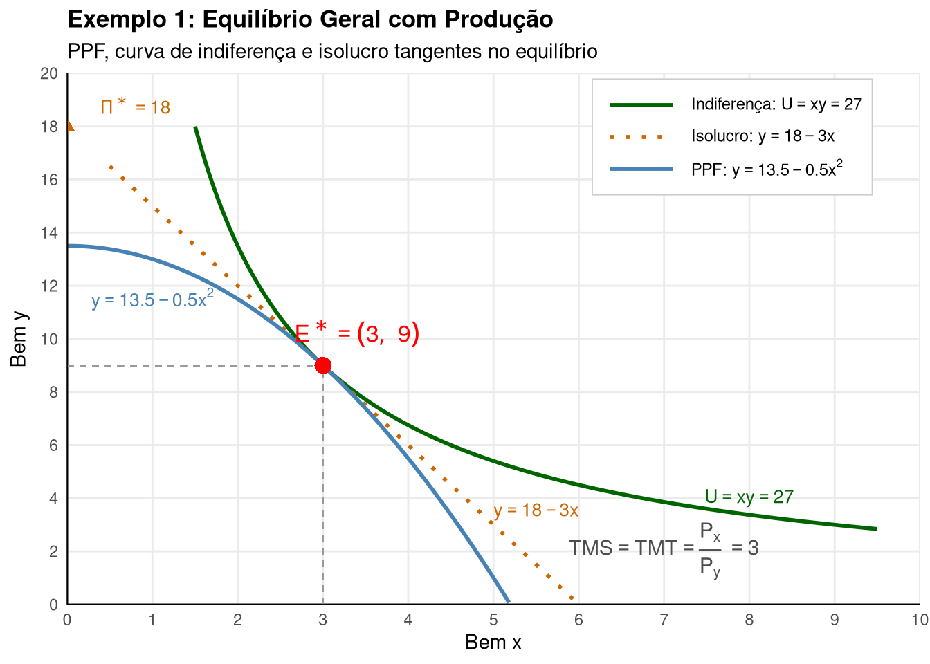
Primeiro Teorema do Bem-Estar: O equilíbrio competitivo é Pareto eficiente. Neste caso, a alocação \((x^*, y^*) = (3, 9)\) maximiza a utilidade do consumidor sujeita à restrição tecnológica.
Condição de tangência: No equilíbrio, a curva de indiferença do consumidor é tangente à PPF, indicando que: \[TMS = TMT = \frac{P_x}{P_y}\]
Papel dos preços: Os preços coordenam as decisões descentralizadas da firma (maximização de lucro) e do consumidor (maximização de utilidade), levando a uma alocação eficiente.
Lei de Walras: A soma dos valores de excesso de demanda em todos os mercados é zero. Se o mercado de \(x\) está em equilíbrio, o mercado de \(y\) também está (podemos verificar apenas \(n-1\) mercados em uma economia com \(n\) bens).
Visualização do Equilíbrio
Para plotar as três curvas no plano \((x, y)\), precisamos transformar cada função de duas variáveis em uma curva, fixando um valor constante e isolando \(y\):
PPF — já está na forma \(y = f(x)\):
\[\begin{aligned}
y &= 13.5 - 0.5x^2 & & \text{fronteira de possibilidades de produção}
\end{aligned}\]
Curva de indiferença — fixar a utilidade no nível de equilíbrio \(U^* = 27\) e isolar \(y\):
\[\begin{aligned}
U(x, y) &= xy = \bar{U} & & \text{função utilidade com } \bar{U} \text{ constante} \\[6pt]
y &= \frac{\bar{U}}{x} = \frac{27}{x} & & \text{isolar } y \text{: curva de indiferença no plano } (x, y)
\end{aligned}\]
Isolucro — fixar o lucro no nível máximo \(\Pi^* = 18\) e isolar \(y\):
\[\begin{aligned}
\Pi &= P_x x + P_y y & & \text{função lucro (receita com dois bens)} \\[6pt]
P_y y &= \Pi^* - P_x x & & \text{isolar o termo em } y \\[6pt]
y &= \frac{\Pi^* - P_x x}{P_y} = \frac{18 - 3x}{1} = 18 - 3x & & \text{reta com intercepto } \Pi^*/P_y \text{ e inclinação } {-P_x/P_y}
\end{aligned}\]
As três curvas são tangentes no ponto de equilíbrio \(E^* = (3, 9)\), onde \(TMS = TMT = P_x/P_y = 3\).
Código
suppressPackageStartupMessages({library(ggplot2)library(latex2exp)})# PPF: y = 13.5 - 0.5x^2x_ppf <-seq(0, 5.2, length.out =300)y_ppf <-13.5-0.5* x_ppf^2# Equilíbriox_eq <-3y_eq <-9U_eq <-27# Curva de indiferença U = xy = 27x_ic <-seq(1.5, 9.5, length.out =300)y_ic <- U_eq / x_ic# Isolucro: y = 18 - 3xx_iso <-seq(0.5, 6, length.out =300)y_iso <-18-3* x_iso# Labels TeX para legendalab_ppf <-TeX("PPF: $y = 13.5 - 0.5x^2$")lab_ic <-TeX("Indiferença: $U = xy = 27$")lab_iso <-TeX("Isolucro: $y = 18 - 3x$")# Dados com aes para legendadados <- dplyr::bind_rows( tibble::tibble(x = x_ppf, y = y_ppf, tipo ="ppf"), tibble::tibble(x = x_ic, y = y_ic, tipo ="ic"), tibble::tibble(x = x_iso, y = y_iso, tipo ="iso"))ggplot2::ggplot(dados, ggplot2::aes(x = x, y = y, color = tipo, linetype = tipo)) + ggplot2::geom_line(linewidth =1) +# Eixos ggplot2::geom_hline(yintercept =0, linewidth =0.5, color ="black") + ggplot2::geom_vline(xintercept =0, linewidth =0.5, color ="black") +# Projeções do equilíbrio ggplot2::geom_segment( ggplot2::aes(x = x_eq, y =0, xend = x_eq, yend = y_eq),linetype ="dashed", color ="gray60", linewidth =0.4, inherit.aes =FALSE ) + ggplot2::geom_segment( ggplot2::aes(x =0, y = y_eq, xend = x_eq, yend = y_eq),linetype ="dashed", color ="gray60", linewidth =0.4, inherit.aes =FALSE ) +# Ponto de equilíbrio ggplot2::geom_point(data = tibble::tibble(x = x_eq, y = y_eq), ggplot2::aes(x = x, y = y),color ="red", size =4, shape =16, inherit.aes =FALSE ) +# Rótulos nas curvas ggplot2::annotate("text", x = x_eq +0.4, y = y_eq +1.2,label =TeX("$E^* = (3,\\, 9)$", output ="character"),color ="red", fontface ="bold", size =4.5, parse =TRUE ) + ggplot2::annotate("text", x =1, y =11.5,label =TeX("$y = 13.5 - 0.5x^2$", output ="character"),color ="steelblue", size =3.5, parse =TRUE ) + ggplot2::annotate("text", x =8, y =4,label =TeX("$U = xy = 27$", output ="character"),color ="darkgreen", size =3.5, parse =TRUE ) + ggplot2::annotate("text", x =5.5, y =3.5,label =TeX("$y = 18 - 3x$", output ="character"),color ="darkorange3", size =3.5, parse =TRUE ) + ggplot2::annotate("text", x =7, y =2,label =TeX("$TMS = TMT = \\frac{P_x}{P_y} = 3$", output ="character"),color ="gray30", size =4, parse =TRUE ) +# Intercepto isolucro ggplot2::geom_point(data = tibble::tibble(x =0, y =18), ggplot2::aes(x = x, y = y),color ="darkorange3", size =2.5, shape =17, inherit.aes =FALSE ) + ggplot2::annotate("text", x =0.8, y =18.8,label =TeX("$\\Pi^* = 18$", output ="character"),color ="darkorange3", size =3.5, parse =TRUE ) +# Escalas com legenda ggplot2::scale_color_manual(values =c("ppf"="steelblue", "ic"="darkgreen", "iso"="darkorange3"),labels =c("ppf"= lab_ppf, "ic"= lab_ic, "iso"= lab_iso) ) + ggplot2::scale_linetype_manual(values =c("ppf"="solid", "ic"="solid", "iso"="dotted"),labels =c("ppf"= lab_ppf, "ic"= lab_ic, "iso"= lab_iso) ) + ggplot2::scale_x_continuous(limits =c(0, 10), expand =c(0, 0),breaks =seq(0, 10, by =1) ) + ggplot2::scale_y_continuous(limits =c(0, 20), expand =c(0, 0),breaks =seq(0, 20, by =2) ) + ggplot2::labs(title ="Exemplo 1: Equilíbrio Geral com Produção",subtitle ="PPF, curva de indiferença e isolucro tangentes no equilíbrio",x =TeX("Bem $x$"), y =TeX("Bem $y$"),color =NULL, linetype =NULL ) + ggplot2::theme_minimal() + ggplot2::theme(legend.position =c(0.78, 0.88),legend.background = ggplot2::element_rect(fill ="white", color ="gray80", linewidth =0.3),legend.text = ggplot2::element_text(size =9),legend.key.width = ggplot2::unit(1.5, "cm"),plot.title = ggplot2::element_text(size =13, face ="bold"),axis.title = ggplot2::element_text(size =11),axis.line = ggplot2::element_line(color ="black", linewidth =0.3),panel.grid.minor = ggplot2::element_blank() )
Note 13.2: Exemplo 2: Um Único Consumidor e Trabalho como Insumo
Estrutura do Modelo
Este exemplo introduz uma característica fundamental das economias reais: o trabalho como insumo produtivo e bem de escolha do consumidor. Considere uma economia com:
Um único consumidor com função utilidade \(U(x,L)\), onde:
\(x\) é o bem de consumo
\(L\) é o trabalho (labor em inglês)
O consumidor valoriza positivamente o consumo de \(x\) e negativamente o trabalho \(L\) (ou equivalentemente, valoriza positivamente o lazer \(1-L\))
Uma dotação inicial de tempo normalizada em 1 unidade (pode-se interpretar como 24 horas, 1 dia, etc.)
O consumidor divide seu tempo entre trabalho \(L\) e lazer \((1-L)\)
Uma firma com função de produção \(x = f(L)\)
A firma transforma trabalho em bem de consumo
O consumidor é proprietário da firma
Dois mercados:
Mercado do bem \(x\) com preço \(P\)
Mercado de trabalho com salário \(w\)
Problema Central: Determinar o salário real de equilíbrio \(\frac{w}{P}\) e as quantidades de equilíbrio \((x^*, L^*)\).
Diferença fundamental em relação ao Exemplo 1: Aqui o insumo (trabalho) é também um argumento da função utilidade do consumidor, criando um trade-off entre consumo e lazer.
Especificação Numérica
Preferências: \[U(x,L) = x(1-L)\]
Esta função captura o trade-off entre consumo (\(x\)) e lazer \((1-L)\). Quanto mais o consumidor trabalha (\(L\) maior), menos lazer tem, reduzindo sua utilidade.
Tecnologia: \[x = f(L) = \sqrt{L}\]
Função de produção com retornos decrescentes de escala (produtividade marginal decrescente do trabalho).
Resolução: Etapa 1 - Problema da Firma
A firma maximiza lucro escolhendo quanto trabalho demandar e quanto bem \(x\) produzir:
\[\begin{aligned}
\Pi(L) &= P\sqrt{L} - wL & & \text{substituindo } x = \sqrt{L} \text{ na função lucro} \\[6pt]
&= \underbrace{P \cdot L^{1/2}}_{f(L)} - \underbrace{w \cdot L}_{g(L)} & & \text{reescrevendo em termos de potências}
\end{aligned}\]
Derivando cada termo em relação a \(L\):
\[\begin{aligned}
\frac{d}{dL}(P \cdot L^{1/2}) &= P \cdot \frac{1}{2} L^{-1/2} = \frac{P}{2\sqrt{L}} & & \text{regra da potência: } \frac{d}{dL}(L^n) = n L^{n-1} \\[6pt]
\frac{d}{dL}(w \cdot L) &= w & & \text{derivada linear}
\end{aligned}\]
Portanto:
\[\begin{aligned}
\frac{d\Pi}{dL} &= \frac{P}{2\sqrt{L}} - w = 0 & & \text{condição de primeira ordem (CPO)} \\[6pt]
\frac{P}{2\sqrt{L}} &= w & & \text{VPMgL = salário} \\[6pt]
\sqrt{L} &= \frac{P}{2w} & & \text{isolando } \sqrt{L} \\[6pt]
L^D &= \frac{P^2}{4w^2} & & \text{demanda de trabalho pela firma}
\end{aligned}\]
Substituindo na função de produção e calculando o lucro:
\[\begin{aligned}
x^S &= \sqrt{L^D} = \frac{P}{2w} & & \text{oferta do bem } x \\[6pt]
\Pi^* &= P \cdot \frac{P}{2w} - w \cdot \frac{P^2}{4w^2} & & \text{substituindo na função lucro} \\[6pt]
&= \frac{P^2}{2w} - \frac{P^2}{4w} = \frac{P^2}{4w} & & \text{lucro máximo}
\end{aligned}\]
Interpretação econômica: A CPO \(\frac{P}{2\sqrt{L}} = w\) diz que a firma demanda trabalho até o ponto onde o valor do produto marginal do trabalho (VPMgL) iguala o salário. O produto marginal é decrescente (\(PMgL = \frac{1}{2\sqrt{L}}\)), então quanto mais trabalho a firma contrata, menor o retorno adicional de cada hora extra.
Resolução: Etapa 2 - Problema do Consumidor
O consumidor maximiza utilidade escolhendo quanto consumir de \(x\) e quanto trabalhar \(L\):
Da restrição orçamentária, \(x = \frac{\Pi^* + wL}{P}\). Substituindo na função utilidade:
\[\begin{aligned}
U(L) &= \frac{\Pi^* + wL}{P}(1-L) & & \text{substituindo } x \text{: problema em uma variável} \\[6pt]
&= \frac{1}{P}\underbrace{(\Pi^* + wL)}_{a + bL}\underbrace{(1-L)}_{1-L} & & \text{produto de duas funções lineares em } L
\end{aligned}\]
\[\begin{aligned}
\frac{dU}{dL} &= \frac{1}{P}[-\Pi^* + w - 2wL] = 0 & & \text{condição de primeira ordem (CPO)} \\[6pt]
-\Pi^* + w &= 2wL & & \text{isolando os termos em } L \\[6pt]
L^S &= \frac{w - \Pi^*}{2w} & & \text{oferta de trabalho}
\end{aligned}\]
Interpretação econômica: O consumidor trabalha até igualar o benefício marginal (salário \(w\)) ao custo marginal (perda de lazer). A presença de \(\Pi^*\) representa o efeito renda: quanto maior o lucro recebido, menor a necessidade de trabalhar.
Resolução: Etapa 3 - Equilíbrio de Mercado
No equilíbrio, a oferta de trabalho iguala a demanda: \(L^S = L^D\).
\[\begin{aligned}
\frac{w - \Pi^*}{2w} &= \frac{P^2}{4w^2} & & \text{igualar oferta e demanda de trabalho} \\[6pt]
\frac{w - \frac{P^2}{4w}}{2w} &= \frac{P^2}{4w^2} & & \text{substituindo } \Pi^* = \frac{P^2}{4w} \\[6pt]
w - \frac{P^2}{4w} &= \frac{P^2}{2w} & & \text{multiplicando por } 2w \\[6pt]
w^2 - \frac{P^2}{4} &= \frac{P^2}{2} & & \text{multiplicando por } w \\[6pt]
w^2 &= \frac{3P^2}{4} & & \text{reagrupando}
\end{aligned}\]
Alocação ótima do tempo: O consumidor trabalha \(\frac{1}{3}\) do tempo disponível e desfruta de \(\frac{2}{3}\) de lazer, equilibrando o trade-off entre renda (para consumir \(x\)) e lazer.
Eficiência produtiva:
\[\begin{aligned}
VPMgL &= P \cdot \frac{1}{2\sqrt{L^*}} = \frac{\sqrt{3}}{2} = w \quad \checkmark & & \text{VPMgL = salário}
\end{aligned}\]
Efeito renda e substituição: O lucro \(\Pi^*\) recebido pelo consumidor reduz sua oferta de trabalho (efeito renda). Se o lucro fosse zero, o consumidor trabalharia mais.
Retornos decrescentes: A produtividade marginal decrescente do trabalho (\(PMgL = \frac{1}{2\sqrt{L}}\)) implica que a firma não demanda trabalho indefinidamente, mesmo com salário baixo.
Propriedades do Equilíbrio
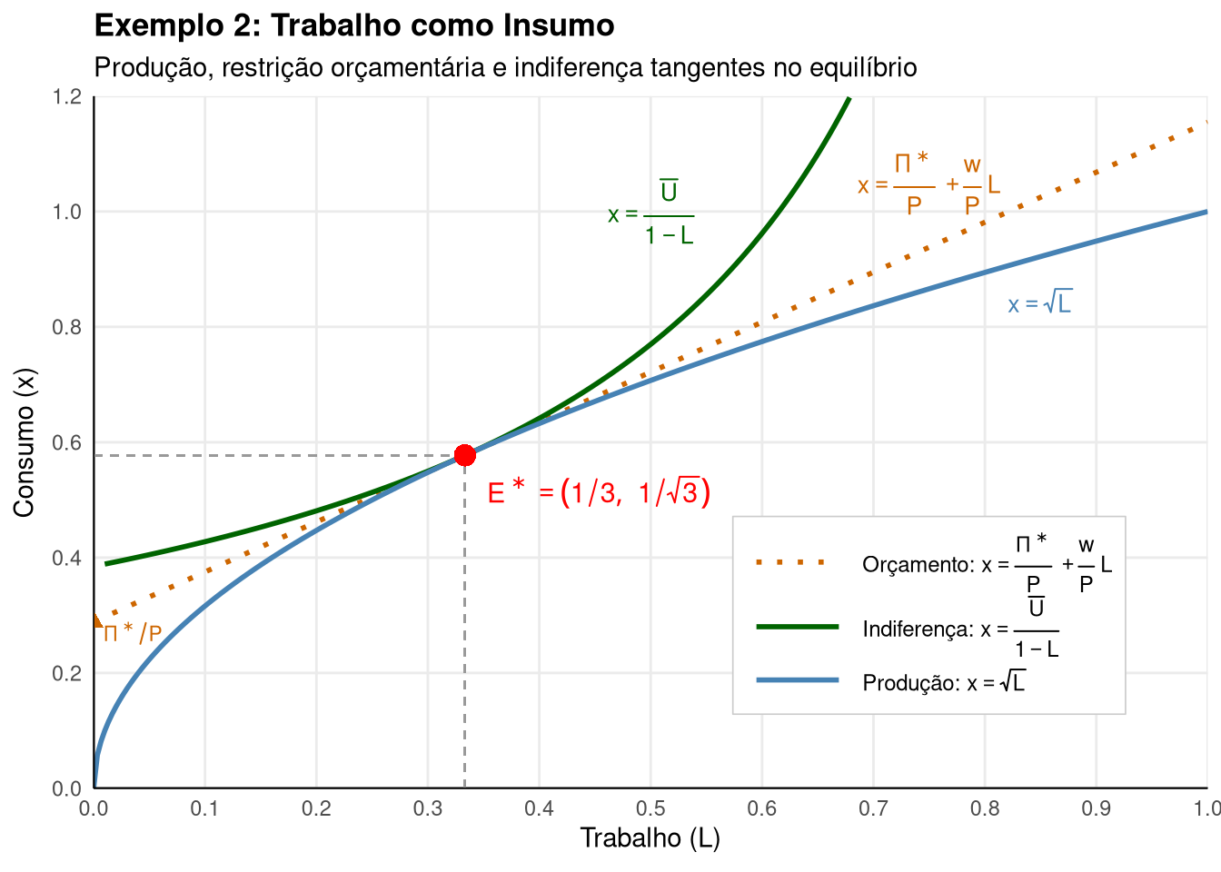
Primeiro Teorema do Bem-Estar: O equilíbrio competitivo é Pareto eficiente. A alocação \((x^*, L^*) = (\frac{1}{\sqrt{3}}, \frac{1}{3})\) maximiza a utilidade do consumidor sujeita à restrição tecnológica e à dotação de tempo.
Papel do salário real: O salário real \(\frac{w}{P}\) coordena as decisões de oferta de trabalho do consumidor e demanda de trabalho da firma, garantindo que o mercado de trabalho esteja em equilíbrio.
Dualidade consumidor-trabalhador: O consumidor desempenha dois papéis: (1) ofertante de trabalho e (2) demandante de bens de consumo. Esses papéis são coordenados através do sistema de preços.
Visualização do Equilíbrio
Para plotar as três curvas no plano \((L, x)\), fixamos os valores de equilíbrio e isolamos \(x\) em função de \(L\):
Função de produção — já está na forma \(x = f(L)\):
\[\begin{aligned}
x &= \sqrt{L} & & \text{função de produção}
\end{aligned}\]
Restrição orçamentária — isolar \(x\):
\[\begin{aligned}
Px &= \Pi^* + wL & & \text{renda = lucro + salário} \\[6pt]
x &= \frac{\Pi^*}{P} + \frac{w}{P} L = \frac{\sqrt{3}}{6} + \frac{\sqrt{3}}{2} L & & \text{reta com intercepto } \Pi^*/P \text{ e inclinação } w/P
\end{aligned}\]
Curva de indiferença — fixar \(U^* = \frac{2\sqrt{3}}{9}\) e isolar \(x\):
\[\begin{aligned}
U(x, L) &= x(1 - L) = \bar{U} & & \text{utilidade constante} \\[6pt]
x &= \frac{\bar{U}}{1 - L} = \frac{2\sqrt{3}/9}{1 - L} & & \text{curva de indiferença no plano } (L, x)
\end{aligned}\]
As três curvas são tangentes no ponto de equilíbrio \(E^* = (1/3, \; 1/\sqrt{3})\).
Código
suppressPackageStartupMessages({library(ggplot2)library(latex2exp)})# Parâmetros de equilíbrioL_eq <-1/3x_eq <-1/sqrt(3)w_P <-sqrt(3)/2pi_star <-sqrt(3)/6U_star <- x_eq * (1- L_eq)# Função de produção x = sqrt(L)L_prod <-seq(0, 1, length.out =300)x_prod <-sqrt(L_prod)# Restrição orçamentária: x = pi*/P + (w/P)*LL_budget <-seq(0, 1, length.out =300)x_budget <- pi_star + w_P * L_budget# Curva de indiferença: x = U*/(1-L)L_ic <-seq(0.01, 0.85, length.out =300)x_ic <- U_star / (1- L_ic)# Labels TeX para legendalab_prod <-TeX("Produção: $x = \\sqrt{L}$")lab_budget <-TeX("Orçamento: $x = \\frac{\\Pi^*}{P} + \\frac{w}{P}L$")lab_ic <-TeX("Indiferença: $x = \\frac{\\bar{U}}{1-L}$")# Dadosdados <- dplyr::bind_rows( tibble::tibble(L = L_prod, x = x_prod, tipo ="prod"), tibble::tibble(L = L_budget, x = x_budget, tipo ="budget"), tibble::tibble(L = L_ic, x = x_ic, tipo ="ic"))ggplot2::ggplot(dados, ggplot2::aes(x = L, y = x, color = tipo, linetype = tipo)) + ggplot2::geom_line(linewidth =1) +# Eixos ggplot2::geom_hline(yintercept =0, linewidth =0.5, color ="black") + ggplot2::geom_vline(xintercept =0, linewidth =0.5, color ="black") +# Projeções do equilíbrio ggplot2::geom_segment( ggplot2::aes(x = L_eq, y =0, xend = L_eq, yend = x_eq),linetype ="dashed", color ="gray60", linewidth =0.4, inherit.aes =FALSE ) + ggplot2::geom_segment( ggplot2::aes(x =0, y = x_eq, xend = L_eq, yend = x_eq),linetype ="dashed", color ="gray60", linewidth =0.4, inherit.aes =FALSE ) +# Ponto de equilíbrio ggplot2::geom_point(data = tibble::tibble(L = L_eq, x = x_eq), ggplot2::aes(x = L, y = x),color ="red", size =4, shape =16, inherit.aes =FALSE ) +# Rótulos ggplot2::annotate("text", x = L_eq +0.12, y = x_eq -0.06,label =TeX("$E^* = (1/3,\\, 1/\\sqrt{3})$", output ="character"),color ="red", fontface ="bold", size =4, parse =TRUE ) + ggplot2::annotate("text", x =0.85, y =0.85,label =TeX("$x = \\sqrt{L}$", output ="character"),color ="steelblue", size =3.5, parse =TRUE ) + ggplot2::annotate("text", x =0.5, y =1,label =TeX("$x = \\frac{\\bar{U}}{1-L}$", output ="character"),color ="darkgreen", size =3.5, parse =TRUE ) + ggplot2::annotate("text", x =0.75, y =1.05,label =TeX("$x = \\frac{\\Pi^*}{P} + \\frac{w}{P}L$", output ="character"),color ="darkorange3", size =3.5, parse =TRUE ) +# Intercepto orçamentário ggplot2::geom_point(data = tibble::tibble(L =0, x = pi_star), ggplot2::aes(x = L, y = x),color ="darkorange3", size =2.5, shape =17, inherit.aes =FALSE ) + ggplot2::annotate("text", x =0.035, y = pi_star -0.019,label =TeX("$\\Pi^*/P$", output ="character"),color ="darkorange3", size =3, parse =TRUE ) +# Escalas com legenda ggplot2::scale_color_manual(values =c("prod"="steelblue", "budget"="darkorange3", "ic"="darkgreen"),labels =c("prod"= lab_prod, "budget"= lab_budget, "ic"= lab_ic) ) + ggplot2::scale_linetype_manual(values =c("prod"="solid", "budget"="dotted", "ic"="solid"),labels =c("prod"= lab_prod, "budget"= lab_budget, "ic"= lab_ic) ) + ggplot2::scale_x_continuous(limits =c(0, 1), expand =c(0, 0),breaks =seq(0, 1, by =0.1) ) + ggplot2::scale_y_continuous(limits =c(0, 1.2), expand =c(0, 0),breaks =seq(0, 1.2, by =0.2) ) + ggplot2::labs(title ="Exemplo 2: Trabalho como Insumo",subtitle ="Produção, restrição orçamentária e indiferença tangentes no equilíbrio",x =TeX("Trabalho ($L$)"), y =TeX("Consumo ($x$)"),color =NULL, linetype =NULL ) + ggplot2::theme_minimal() + ggplot2::theme(legend.position =c(0.75, 0.25),legend.background = ggplot2::element_rect(fill ="white", color ="gray80", linewidth =0.3),legend.text = ggplot2::element_text(size =9),legend.key.width = ggplot2::unit(1.5, "cm"),plot.title = ggplot2::element_text(size =13, face ="bold"),axis.title = ggplot2::element_text(size =11),axis.line = ggplot2::element_line(color ="black", linewidth =0.3),panel.grid.minor = ggplot2::element_blank() )
Note 13.3: Exemplo 3: Dois Consumidores e Trabalho como Insumo
Estrutura do Modelo
Considere uma economia com:
2 consumidores: \(A\) e \(B\) com preferências heterogêneas
Trabalho como insumo produtivo
Uma firma que produz o bem \(X\) usando trabalho
Preferências:
Consumidor A (gosta de lazer): \(U_A (X_A, L_A) = X_A (1 - L_A)\)
Consumidor B (não valoriza lazer): \(U_B (X_B, L_B) = X_B\)
Dotações: Cada consumidor possui 1 unidade de tempo.
Tecnologia: \(X_F = \sqrt{L_F}\) onde \(L_F = L_A + L_B\)
Propriedade: O consumidor \(B\) é proprietário da firma e recebe o lucro \(\Pi\).
Resolução: Etapa 1 - Problema da Firma
A firma tem a mesma função de produção \(X = \sqrt{L}\) do Note 13.2. A diferença é que agora o trabalho total é \(L_F = L_A + L_B\) (dois ofertantes). O problema da firma e suas soluções são idênticos:
O consumidor A tem a mesma função utilidade \(U = X(1-L)\) do Note 13.2, mas com uma diferença crucial: não recebe lucro (a firma pertence a B). Sua renda é apenas o salário.
\[\begin{aligned}
\max_{X_A, L_A} \; U_A &= X_A(1-L_A) & & \text{mesma utilidade do Ex. 2} \\[6pt]
\text{s.a.} \quad P X_A &= w L_A & & \text{renda = apenas salário (sem } \Pi\text{)}
\end{aligned}\]
A resolução segue a mesma lógica do Note 13.2 (ver derivadas detalhadas lá):
\[\begin{aligned}
\frac{dU_A}{dL_A} &= \frac{w}{P}[1 - 2L_A] = 0 & & \text{CPO: mesma forma do Ex. 2} \\[6pt]
L_A &= \frac{1}{2} & & \text{oferta de trabalho de A} \\[6pt]
X_A &= \frac{w}{2P} & & \text{demanda do bem } X \text{ por A}
\end{aligned}\]
Interpretação econômica: O consumidor A trabalha exatamente metade do tempo disponível, independentemente dos preços! Isso ocorre porque \(U_A = X_A(1-L_A)\) é Cobb-Douglas com expoentes iguais, implicando alocação igual entre trabalho e lazer. Note que, diferentemente do Note 13.2, a ausência de lucro \(\Pi\) não altera \(L_A\) neste caso (no Note 13.2, \(\Pi\) aparecia na oferta de trabalho \(L^S = \frac{w - \Pi^*}{2w}\), mas aqui \(\Pi = 0\) para A, dando o mesmo resultado \(L_A = 1/2\)).
Resolução: Etapa 3 - Problema do Consumidor B
Aqui está a novidade deste exemplo: o consumidor B tem preferências radicalmente diferentes de A.
\[\begin{aligned}
\max_{X_B, L_B} \; U_B &= X_B & & \text{utilidade linear: lazer não entra!} \\[6pt]
\text{s.a.} \quad P X_B &= w L_B + \Pi & & \text{renda = salário + lucro (proprietário da firma)}
\end{aligned}\]
Como \(U_B = X_B\), o consumidor B quer maximizar \(X_B = \frac{w L_B + \Pi}{P}\). Não há CPO interior: a utilidade marginal do lazer é zero (\(\frac{\partial U_B}{\partial (1-L_B)} = 0\)), então cada hora adicional de trabalho sempre aumenta a utilidade via mais consumo. A solução é de canto:
\[\begin{aligned}
L_B &= 1 & & \text{solução de canto: trabalha toda a dotação de tempo} \\[6pt]
X_B &= \frac{w + \Pi}{P} & & \text{demanda do bem } X \text{ por B}
\end{aligned}\]
Interpretação econômica: B não valoriza lazer, então trabalha o máximo possível. Além disso, como proprietário da firma, recebe \(\Pi\) — sua renda total (\(wL_B + \Pi\)) é substancialmente maior que a de A (\(wL_A\)).
Resolução: Etapa 4 - Equilíbrio de Mercado
No equilíbrio, a oferta agregada deve igualar a demanda agregada em ambos os mercados.
B consome 5 vezes mais que A: trabalha o dobro e recebe todo o lucro (\(\Pi = 1{,}5\), ou 60% de sua renda)
Papel da propriedade da firma: A propriedade cria desigualdade de renda mesmo com salários iguais. Se fosse dividida igualmente, a distribuição seria mais equitativa.
Eficiência alocativa: O equilíbrio é Pareto eficiente — não é possível melhorar a situação de um consumidor sem piorar a do outro.
Preço relativo: \(\frac{P}{w} = \sqrt{6} \approx 2{,}449\) — são necessárias \(\sqrt{6}\) unidades de salário para comprar 1 unidade de \(X\), refletindo a produtividade decrescente.
Propriedades do Equilíbrio
Primeiro Teorema do Bem-Estar: O equilíbrio competitivo é Pareto eficiente. A alocação \((X_A, L_A, X_B, L_B) = (0.204, 0.5, 1.021, 1)\) maximiza a utilidade de cada consumidor sujeita às restrições tecnológicas, orçamentárias e de dotação de tempo.
Papel dos preços: Os preços \((P, w)\) coordenam as decisões descentralizadas da firma (maximização de lucro) e dos consumidores (maximização de utilidade), levando a uma alocação eficiente.
Heterogeneidade e agregação: Mesmo com preferências heterogêneas, o sistema de preços coordena as decisões individuais, garantindo que a oferta agregada iguale a demanda agregada em todos os mercados.
Lei de Walras: A soma dos valores de excesso de demanda em todos os mercados é zero. Se o mercado de trabalho está em equilíbrio, o mercado do bem \(X\) também está (verificamos apenas \(n-1\) mercados em uma economia com \(n\) bens).
Note 13.4: Exemplo 4: Dois Consumidores e Dotações Iniciais Positivas
Estrutura do Modelo
Este exemplo introduz uma nova característica fundamental: dotações iniciais positivas de bens e um bem de consumo como insumo produtivo. Considere uma economia com:
2 consumidores: \(A\) e \(B\) com preferências Cobb-Douglas idênticas
2 bens de consumo: \(x\) e \(y\)
Dotações iniciais heterogêneas:
Consumidor A: \(\omega_A = (0, 4)\) — possui apenas bem \(y\)
Consumidor B: \(\omega_B = (2, 0)\) — possui apenas bem \(x\)
Uma firma que produz bem \(x\) usando bem \(y\) como insumo
Propriedade: O consumidor B é proprietário da firma e recebe o lucro \(\Pi\)
Diferença fundamental em relação aos exemplos anteriores: Aqui não há trabalho como insumo. A firma transforma um bem de consumo (\(y\)) em outro bem de consumo (\(x\)). Os consumidores possuem dotações iniciais de bens que podem consumir ou vender.
Especificação Numérica
Preferências (Cobb-Douglas):
\[U_A(x_A, y_A) = x_A y_A\]
\[U_B(x_B, y_B) = x_B y_B\]
Dotações iniciais:
\[\omega_A = (0, 4) \quad \text{(4 unidades do bem } y)\]
\[\omega_B = (2, 0) \quad \text{(2 unidades do bem } x)\]
Tecnologia:
\[X_F = \sqrt{y_F}\]
onde \(X_F\) é a produção do bem \(x\) e \(y_F\) é o insumo do bem \(y\).
Propriedade: O consumidor B recebe todo o lucro \(\Pi\) da firma.
Resolução: Etapa 1 - Problema da Firma
A firma tem a mesma função de produção \(\sqrt{\cdot}\) dos exemplos anteriores, mas agora o insumo é o bem \(y\) (um bem de consumo), não trabalho. Isso significa que a firma compete com os consumidores pelo bem \(y\) — criando um trade-off entre consumo direto e uso produtivo.
\[\begin{aligned}
\max_{y_F} \; \Pi(y_F) &= P_x \sqrt{y_F} - P_y y_F & & \text{mesma estrutura dos Ex. 2-3, com } y_F \text{ no lugar de } L \\[6pt]
\frac{d\Pi}{dy_F} &= \frac{P_x}{2\sqrt{y_F}} - P_y = 0 & & \text{CPO: VPMg}_y = P_y \\[6pt]
y_F &= \frac{P_x^2}{4P_y^2} & & \text{demanda de insumo } y \\[6pt]
X_F &= \frac{P_x}{2P_y}, \quad \Pi = \frac{P_x^2}{4P_y} & & \text{oferta e lucro máximo}
\end{aligned}\]
Resolução: Etapas 2 e 3 - Problemas dos Consumidores
Ambos os consumidores têm \(U = xy\) (mesma utilidade do Note 13.1), portanto aplicam a regra “metade da renda em cada bem” (ver derivação no Note 13.1). A novidade aqui são as rendas diferentes: dotações heterogêneas e lucro assimétrico.
Consumidor A — dotação \(\omega_A = (0, 4)\), renda \(M_A = 4P_y\), não recebe lucro:
\[\begin{aligned}
x_A &= \frac{M_A}{2P_x} = \frac{2P_y}{P_x} & & \text{vende metade de } y \text{ para comprar } x \\[6pt]
y_A &= \frac{M_A}{2P_y} = 2 & & \text{consome metade de sua dotação de } y
\end{aligned}\]
Consumidor B — dotação \(\omega_B = (2, 0)\), renda \(M_B = 2P_x + \Pi\) (recebe todo o lucro):
\[\begin{aligned}
x_B &= \frac{M_B}{2P_x} = 1 + \frac{\Pi}{2P_x} & & \text{retém parte de } x \text{ e usa lucro para comprar mais} \\[6pt]
y_B &= \frac{M_B}{2P_y} = \frac{P_x}{P_y} + \frac{P_x^2}{8P_y^2} & & \text{compra } y \text{ com renda de dotação + lucro}
\end{aligned}\]
Note que B não possui \(y\) na dotação, mas a firma produz \(x\) usando \(y\) como insumo — B financia sua compra de \(y\) vendendo parte de sua dotação de \(x\) e recebendo \(\Pi\).
Dotações iniciais e comércio: A vende \(y\) para comprar \(x\); B vende \(x\) para comprar \(y\); a firma compra \(y\) (\(\frac{4}{9}\)) para produzir \(x\) (\(\frac{2}{3}\)). O comércio permite que ambos consumam ambos os bens.
Papel da produção: A firma aumenta a oferta de \(x\) de 2 para \(\frac{8}{3}\) e reduz a oferta disponível de \(y\) de 4 para \(\frac{32}{9}\).
Distribuição de renda: A tem maior renda (4 vs 3,111) devido à dotação inicial maior, mas B recebe lucro adicional (\(\Pi = 0{,}444\), +14% de renda).
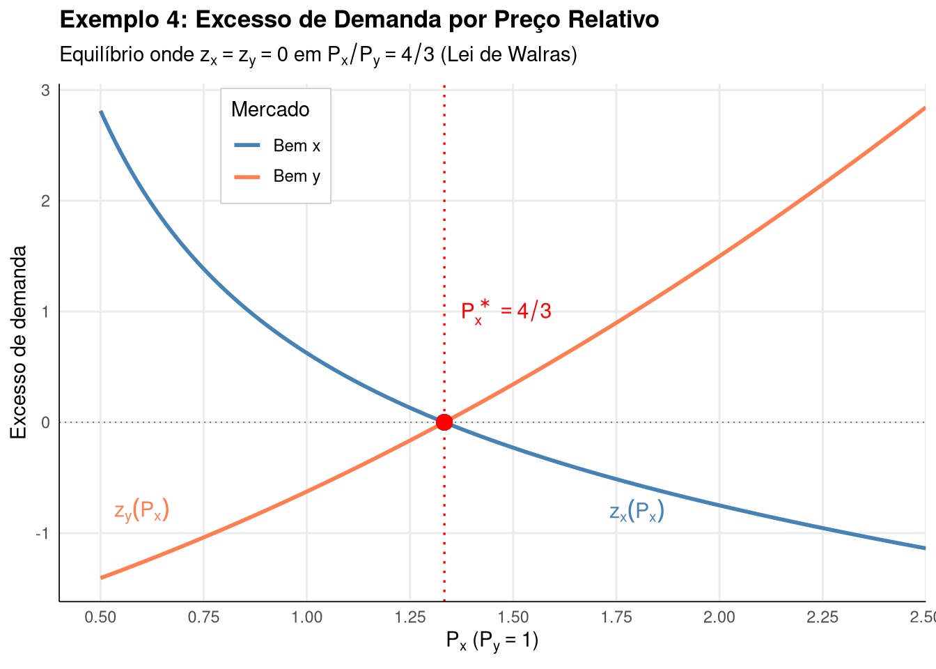
Preço relativo: \(\frac{P_x}{P_y} = \frac{4}{3}\) reflete a escassez relativa de \(x\) (dotação total de apenas 2 unidades).
Eficiência alocativa:
\[\begin{aligned}
TMS_A &= \frac{y_A}{x_A} = \frac{2}{3/2} = \frac{4}{3} = \frac{P_x}{P_y} \quad \checkmark & & \text{TMS de A = razão de preços} \\[6pt]
TMS_B &= \frac{y_B}{x_B} = \frac{14/9}{7/6} = \frac{4}{3} = \frac{P_x}{P_y} \quad \checkmark & & \text{TMS de B = razão de preços} \\[6pt]
TMT &= 2\sqrt{y_F} = 2\sqrt{4/9} = \frac{4}{3} = \frac{P_x}{P_y} \quad \checkmark & & \text{TMT = razão de preços}
\end{aligned}\]
Como \(TMS_A = TMS_B = TMT\), a alocação é Pareto eficiente (Primeiro Teorema do Bem-Estar).
Propriedades do Equilíbrio
A alocação \((x_A, y_A, x_B, y_B) = (1{,}5; \; 2; \; 1{,}167; \; 1{,}556)\) é Pareto eficiente, satisfazendo as três condições de eficiência simultaneamente (eficiência na troca, na produção e na composição do produto — ver Note 13.8).
Segundo Teorema do Bem-Estar: A distribuição de bem-estar depende das dotações iniciais e da propriedade da firma. Mudanças nessas distribuições alteram o equilíbrio, mas mantêm a eficiência — qualquer alocação Pareto eficiente pode ser alcançada com redistribuições adequadas.
Visualização: Fluxos de Equilíbrio
Código
suppressPackageStartupMessages({library(ggplot2)library(latex2exp)})# Parâmetros: Py=1, Px=4/3Px <-4/3Py <-1Pi_val <- Px^2/ (4* Py) # 4/9# Excesso de demanda no mercado de x como função de Pxpx_range <-seq(0.5, 2.5, length.out =300)# Oferta: 2 + px/2# Demanda: 2/px + 1 + px/8excesso_x <- (2/px_range +1+ px_range/8) - (2+ px_range/2)# Excesso de demanda no mercado de y# Oferta: 4# Demanda: 2 + px + px^2/8 + px^2/4excesso_y <- (2+ px_range + px_range^2/8+ px_range^2/4) -4dados <- dplyr::bind_rows( tibble::tibble(px = px_range, excesso = excesso_x, mercado ="x"), tibble::tibble(px = px_range, excesso = excesso_y, mercado ="y"))lab_x <-TeX("Bem $x$")lab_y <-TeX("Bem $y$")ggplot2::ggplot(dados, ggplot2::aes(x = px, y = excesso, color = mercado, linetype = mercado)) + ggplot2::geom_line(linewidth =1) +# Linha de referência (excesso de demanda = 0) ggplot2::geom_hline(yintercept =0, linewidth =0.3, color ="gray40", linetype ="dotted") +# Linha do equilíbrio ggplot2::geom_vline(xintercept = Px, linetype ="dotted", color ="red", linewidth =0.6) +# Ponto de equilíbrio ggplot2::geom_point(data = tibble::tibble(px = Px, excesso =0), ggplot2::aes(x = px, y = excesso),color ="red", size =4, shape =16, inherit.aes =FALSE ) +# Rótulos ggplot2::annotate("text", x = Px +0.15, y =1,label =TeX("$P_x^* = 4/3$", output ="character"),color ="red", fontface ="bold", size =4, parse =TRUE ) + ggplot2::annotate("text", x =1.8, y =-0.8,label =TeX("$z_x(P_x)$", output ="character"),color ="steelblue", size =4, parse =TRUE ) + ggplot2::annotate("text", x =0.6, y =-0.8,label =TeX("$z_y(P_x)$", output ="character"),color ="coral", size =4, parse =TRUE ) +# Escalas ggplot2::scale_color_manual(values =c("x"="steelblue", "y"="coral"),labels =c("x"= lab_x, "y"= lab_y) ) + ggplot2::scale_linetype_manual(values =c("x"="solid", "y"="solid"),labels =c("x"= lab_x, "y"= lab_y) ) + ggplot2::scale_x_continuous(limits =c(0.4, 2.5), expand =c(0, 0),breaks =seq(0.5, 2.5, by =0.25) ) + ggplot2::labs(title ="Exemplo 4: Excesso de Demanda por Preço Relativo",subtitle =TeX("Equilíbrio onde $z_x = z_y = 0$ em $P_x/P_y = 4/3$ (Lei de Walras)"),x =TeX("$P_x$ ($P_y = 1$)"),y ="Excesso de demanda",color ="Mercado", linetype ="Mercado" ) + ggplot2::theme_minimal() + ggplot2::theme(legend.position =c(0.25, 0.88),legend.background = ggplot2::element_rect(fill ="white", color ="gray80", linewidth =0.3),legend.text = ggplot2::element_text(size =9),plot.title = ggplot2::element_text(size =13, face ="bold"),axis.title = ggplot2::element_text(size =11),axis.line = ggplot2::element_line(color ="black", linewidth =0.3),panel.grid.minor = ggplot2::element_blank() )
Note 13.5: Exemplo 5: Comida como Insumo Produtivo e Bem de Consumo
Estrutura do Modelo
Este exemplo combina elementos dos Note 13.1 e Note 13.4: dois consumidores idênticos com Cobb-Douglas, uma firma com \(\sqrt{\cdot}\), mas com uma característica nova — o bem Comida exerce papel duplo: é simultaneamente bem de consumo e insumo produtivo.
2 consumidores (Ana e Bruno) com preferências idênticas: \(U(C, R) = C^{0{,}5} R^{0{,}5}\)
2 bens: Comida (\(C\)) e Roupa (\(R\))
Dotações: cada consumidor possui 10 unidades de Comida e 0 de Roupa
Firma: produz Roupa usando Comida como insumo: \(R = 2\sqrt{C_f}\)
Propriedade: cada consumidor recebe metade do lucro (\(\Pi/2\))
Diferença fundamental: nos exemplos anteriores, o insumo era trabalho (que não é um bem de mercado com oferta fixa) ou um bem separado. Aqui, a firma compete com os consumidores pela Comida — cada unidade de Comida usada como insumo é uma unidade a menos disponível para consumo.
Resolução: Etapa 1 - Problema da Firma
A firma tem a mesma estrutura \(\sqrt{\cdot}\) dos Ex. 2-4, mas agora o insumo é Comida (\(C_f\)) e o produto é Roupa (\(R\)):
Ana e Bruno têm \(U = C^{0{,}5} R^{0{,}5}\) (mesma regra “metade da renda em cada bem” do Note 13.1). A novidade é que a renda inclui a parcela do lucro:
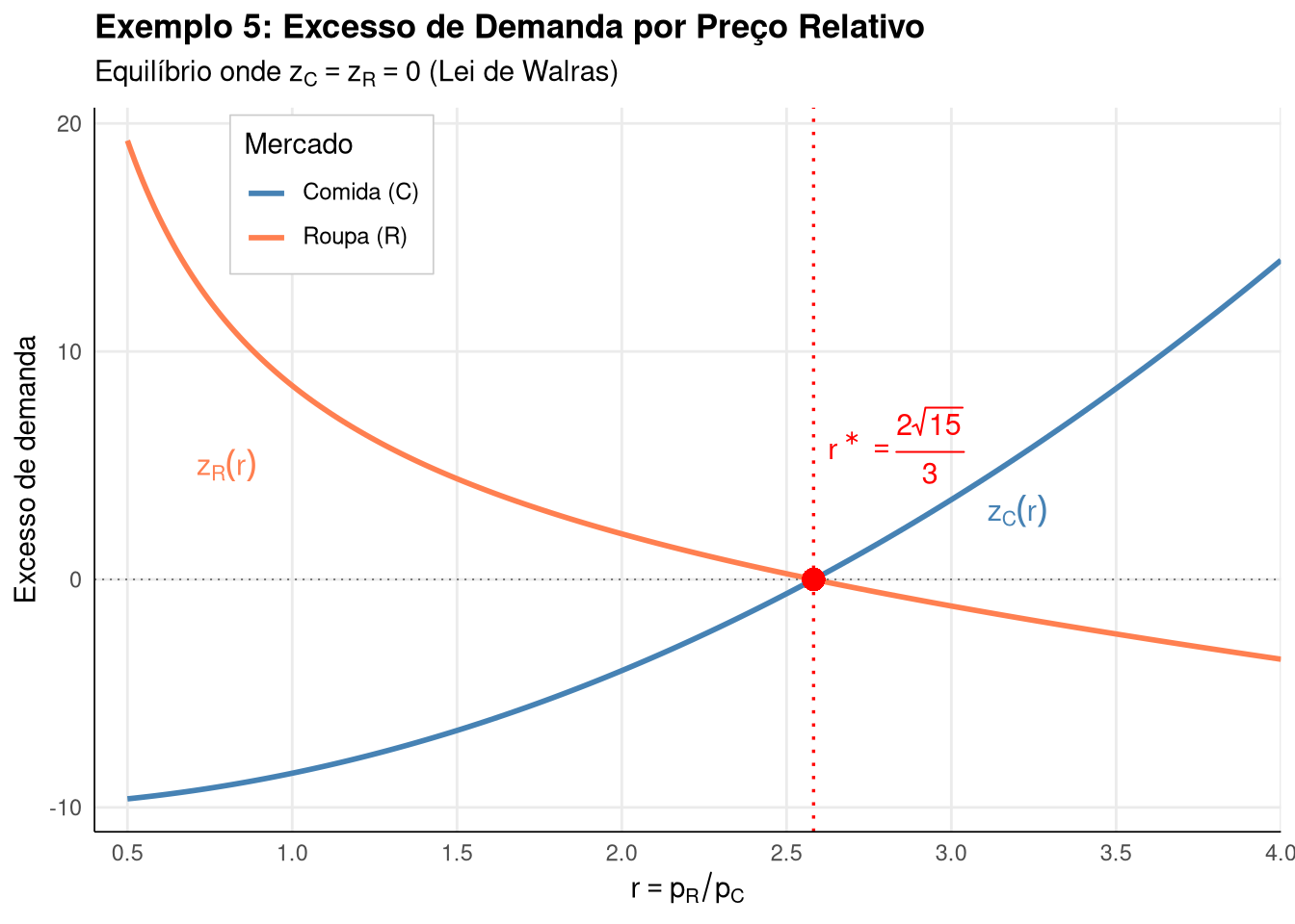
Preço relativo: \(p_R/p_C \approx 2{,}582\) — cada unidade de roupa custa ~2,6 unidades de comida, refletindo o custo de oportunidade do uso da comida como insumo.
Insumo produtivo: \(\frac{20}{3}\) unidades (\(\frac{1}{3}\) da dotação total)
Distribuição de renda: Renda de dotação = \(10\) (76%), Renda de lucro = \(\frac{10}{3}\) (24%). A distribuição dos lucros é essencial — ignorá-la produz preços e quantidades incorretos (ver discussão na introdução deste exemplo).
Expansão das possibilidades de consumo: Sem produção, os consumidores teriam apenas comida e utilidade zero (\(R = 0 \Rightarrow U = 0\)). A firma permite acessar roupa, expandindo o bem-estar.
Visualização do Equilíbrio
Código
suppressPackageStartupMessages({library(ggplot2)library(latex2exp)})# Preço relativo de equilíbrior_eq <-sqrt(20/3)r_range <-seq(0.5, 4, length.out =300)# Excesso de demanda (com lucro distribuído)excesso_comida <-10+3* r_range^2/2-20excesso_roupa <- (10+ r_range^2/2) / r_range -2* r_rangedados <- dplyr::bind_rows( tibble::tibble(r = r_range, excesso = excesso_comida, mercado ="comida"), tibble::tibble(r = r_range, excesso = excesso_roupa, mercado ="roupa"))lab_c <-TeX("Comida ($C$)")lab_r <-TeX("Roupa ($R$)")ggplot2::ggplot(dados, ggplot2::aes(x = r, y = excesso, color = mercado)) + ggplot2::geom_line(linewidth =1) +# Linha de referência ggplot2::geom_hline(yintercept =0, linewidth =0.3, color ="gray40", linetype ="dotted") +# Linha do equilíbrio ggplot2::geom_vline(xintercept = r_eq, linetype ="dotted", color ="red", linewidth =0.6) +# Ponto de equilíbrio ggplot2::geom_point(data = tibble::tibble(r = r_eq, excesso =0), ggplot2::aes(x = r, y = excesso),color ="red", size =4, shape =16, inherit.aes =FALSE ) +# Rótulos ggplot2::annotate("text", x = r_eq +0.25, y =6,label =TeX("$r^* = \\frac{2\\sqrt{15}}{3}$", output ="character"),color ="red", fontface ="bold", size =4, parse =TRUE ) + ggplot2::annotate("text", x =3.2, y =3,label =TeX("$z_C(r)$", output ="character"),color ="steelblue", size =4, parse =TRUE ) + ggplot2::annotate("text", x =0.8, y =5,label =TeX("$z_R(r)$", output ="character"),color ="coral", size =4, parse =TRUE ) +# Escalas ggplot2::scale_color_manual(values =c("comida"="steelblue", "roupa"="coral"),labels =c("comida"= lab_c, "roupa"= lab_r) ) + ggplot2::scale_x_continuous(limits =c(0.4, 4), expand =c(0, 0),breaks =seq(0.5, 4, by =0.5) ) + ggplot2::labs(title ="Exemplo 5: Excesso de Demanda por Preço Relativo",subtitle =TeX("Equilíbrio onde $z_C = z_R = 0$ (Lei de Walras)"),x =TeX("$r = p_R / p_C$"),y ="Excesso de demanda",color ="Mercado" ) + ggplot2::theme_minimal() + ggplot2::theme(legend.position =c(0.2, 0.88),legend.background = ggplot2::element_rect(fill ="white", color ="gray80", linewidth =0.3),legend.text = ggplot2::element_text(size =9),plot.title = ggplot2::element_text(size =13, face ="bold"),axis.title = ggplot2::element_text(size =11),axis.line = ggplot2::element_line(color ="black", linewidth =0.3),panel.grid.minor = ggplot2::element_blank() )
Note 13.6: Fronteira de Possibilidades de Produção (PPF)
Conceito
A Fronteira de Possibilidades de Produção (PPF, ou FPP) descreve o conjunto de combinações de bens que uma economia pode produzir, dadas suas restrições tecnológicas e de recursos (Varian, 2012). A PPF é a fronteira do conjunto de possibilidades de produção — o conjunto de todas as combinações factíveis de produtos.
A inclinação da PPF é a Taxa Marginal de Transformação (TMT), que mede o custo de oportunidade de produzir uma unidade adicional de um bem em termos do outro.
Construção da PPF com Tecnologias Lineares
Considere uma economia com:
Um trabalhador com \(\bar{L} = 10\) horas disponíveis
Dois bens: peixes (\(F\)) e cocos (\(C\))
Tecnologias lineares:
\(F = 10 L_F\) (10 peixes por hora)
\(C = 20 L_C\) (20 cocos por hora)
Restrição de recurso: \(L_F + L_C = \bar{L} = 10\)
Derivação da PPF
\[\begin{aligned}
L_F &= \frac{F}{10}, \quad L_C = \frac{C}{20} & & \text{inverter as funções de produção} \\[6pt]
\frac{F}{10} + \frac{C}{20} &= 10 & & \text{substituir na restrição de recurso} \\[6pt]
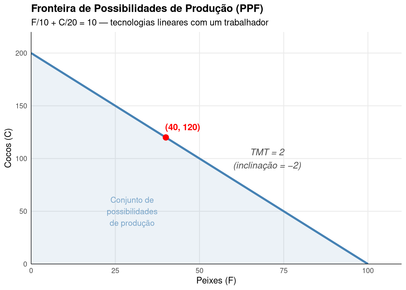
C &= 200 - 2F & & \text{PPF linear}
\end{aligned}\]
Interpretação: Para produzir 1 peixe adicional, é necessário sacrificar 2 cocos. Isso ocorre porque:
1 peixe requer \(\frac{1}{10}\) hora de trabalho
Essa hora produziria \(20 \times \frac{1}{10} = 2\) cocos
A TMT é constante porque as tecnologias são lineares (retornos constantes de escala com um único insumo).
Visualização
Código
suppressPackageStartupMessages({library(ggplot2)})# PPF: C = 200 - 2FF_vals <-seq(0, 100, length.out =200)C_vals <-200-2* F_vals# Ponto exemploF_ex <-40C_ex <-200-2* F_exggplot2::ggplot() + ggplot2::geom_line(data = tibble::tibble(F = F_vals, C = C_vals), ggplot2::aes(x = F, y = C),color ="steelblue", linewidth =1.2 ) + ggplot2::geom_ribbon(data = tibble::tibble(F = F_vals, C = C_vals), ggplot2::aes(x = F, ymin =0, ymax = C),fill ="steelblue", alpha =0.1 ) + ggplot2::geom_point(data = tibble::tibble(F = F_ex, C = C_ex), ggplot2::aes(x = F, y = C),color ="red", size =3 ) + ggplot2::annotate("text", x = F_ex +5, y = C_ex +10,label =paste0("(", F_ex, ", ", C_ex, ")"),color ="red", fontface ="bold" ) + ggplot2::annotate("text", x =70, y =100,label ="TMT = 2\n(inclinação = −2)",color ="gray30", size =4, fontface ="italic" ) + ggplot2::annotate("text", x =30, y =50,label ="Conjunto de\npossibilidades\nde produção",color ="steelblue", size =3.5, alpha =0.7 ) + ggplot2::labs(title ="Fronteira de Possibilidades de Produção (PPF)",subtitle ="F/10 + C/20 = 10 — tecnologias lineares com um trabalhador",x ="Peixes (F)", y ="Cocos (C)" ) + ggplot2::scale_x_continuous(limits =c(0, 110), expand =c(0, 0)) + ggplot2::scale_y_continuous(limits =c(0, 220), expand =c(0, 0)) + ggplot2::theme_minimal() + ggplot2::theme(plot.title = ggplot2::element_text(size =13, face ="bold"),axis.title = ggplot2::element_text(size =11),axis.line = ggplot2::element_line(color ="black", linewidth =0.3),panel.grid.minor = ggplot2::element_blank() )
Propriedades da PPF
Inclinação negativa: Produzir mais de um bem requer sacrificar o outro (custo de oportunidade).
Forma: Com tecnologias lineares e um insumo, a PPF é uma reta. Com retornos decrescentes ou múltiplos insumos, a PPF é côncava (convexa em relação à origem).
Pontos na fronteira: Representam alocações eficientes na produção — todos os recursos estão sendo utilizados.
Pontos interiores: Representam ineficiência produtiva — há recursos ociosos.
Pontos exteriores: São tecnologicamente inviáveis com os recursos disponíveis.
Note 13.7: Vantagem Comparativa e PPF Conjunta
Conceito
Quando uma economia possui múltiplos trabalhadores com produtividades diferentes, a PPF conjunta reflete a especialização ótima baseada na vantagem comparativa(Varian, 2012).
Um trabalhador tem vantagem comparativa na produção de um bem se seu custo de oportunidade de produzir esse bem é menor do que o do outro trabalhador.
Especificação
Dois trabalhadores, cada um com 10 horas:
Peixes/hora
Cocos/hora
TMT (cocos por peixe)
Robinson
10
20
2
Friday
20
10
0,5
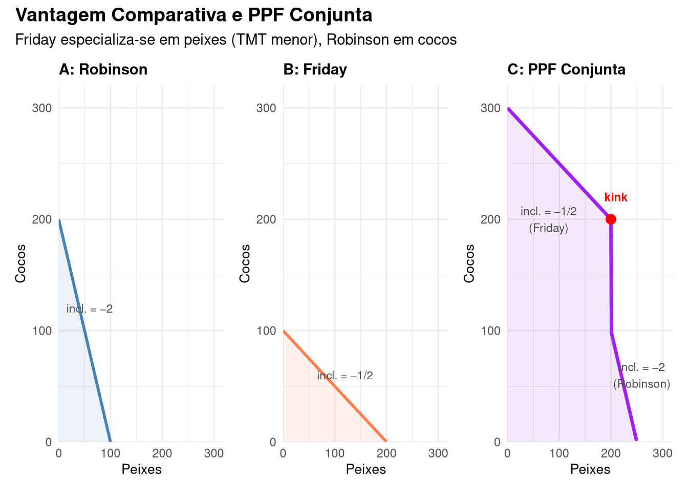
Robinson tem vantagem comparativa em cocos (TMT = 2: sacrifica apenas 0,5 peixe por coco).
Friday tem vantagem comparativa em peixes (TMT = 0,5: sacrifica apenas 0,5 coco por peixe).
Primeiro, Friday vai para peixes (vantagem comparativa): cada peixe de Friday custa apenas 0,5 coco. Friday produz até \(F_F = 200\) peixes, restando \(C = 300 - 100 = 200\) cocos (apenas de Robinson).
Depois, Robinson vai para peixes: cada peixe de Robinson custa 2 cocos. Robinson produz até \(F_R = 100\) peixes adicionais.
Máximo de peixes: \(F_{max} = 200 + 100 = 300\)
A PPF conjunta tem um kink em \((F, C) = (200, 200)\):
\[
C = \begin{cases} 300 - \frac{1}{2}F & \text{se } 0 \leq F \leq 200 \\ 500 - 2F & \text{se } 200 \leq F \leq 300 \end{cases}
\]
Visualização
Código
suppressPackageStartupMessages({library(ggplot2)library(dplyr)library(patchwork)})# PPF Robinson: C = 200 - 2F, F in [0, 100]F_R <-seq(0, 100, length.out =100)C_R <-200-2* F_R# PPF Friday: C = 100 - 0.5F, F in [0, 200]F_F <-seq(0, 200, length.out =100)C_F <-100-0.5* F_F# PPF ConjuntaF_J1 <-seq(0, 200, length.out =100)C_J1 <-300-0.5* F_J1F_J2 <-seq(200, 300, length.out =100)C_J2 <-500-2* F_J2F_J <-c(F_J1, F_J2[-1])C_J <-c(C_J1, C_J2[-1])tema <- ggplot2::theme_minimal() + ggplot2::theme(plot.title = ggplot2::element_text(size =11, face ="bold"),axis.title = ggplot2::element_text(size =10) )p1 <- ggplot2::ggplot(tibble::tibble(F = F_R, C = C_R), ggplot2::aes(x = F, y = C)) + ggplot2::geom_line(color ="steelblue", linewidth =1) + ggplot2::geom_ribbon(ggplot2::aes(ymin =0, ymax = C), fill ="steelblue", alpha =0.1) + ggplot2::annotate("text", x =60, y =120, label ="incl. = −2", color ="gray30", size =3) + ggplot2::labs(title ="A: Robinson", x ="Peixes", y ="Cocos") + ggplot2::scale_x_continuous(limits =c(0, 320), expand =c(0, 0)) + ggplot2::scale_y_continuous(limits =c(0, 320), expand =c(0, 0)) + temap2 <- ggplot2::ggplot(tibble::tibble(F = F_F, C = C_F), ggplot2::aes(x = F, y = C)) + ggplot2::geom_line(color ="coral", linewidth =1) + ggplot2::geom_ribbon(ggplot2::aes(ymin =0, ymax = C), fill ="coral", alpha =0.1) + ggplot2::annotate("text", x =120, y =60, label ="incl. = −1/2", color ="gray30", size =3) + ggplot2::labs(title ="B: Friday", x ="Peixes", y ="Cocos") + ggplot2::scale_x_continuous(limits =c(0, 320), expand =c(0, 0)) + ggplot2::scale_y_continuous(limits =c(0, 320), expand =c(0, 0)) + temap3 <- ggplot2::ggplot(tibble::tibble(F = F_J, C = C_J), ggplot2::aes(x = F, y = C)) + ggplot2::geom_line(color ="purple", linewidth =1.2) + ggplot2::geom_ribbon(ggplot2::aes(ymin =0, ymax = C), fill ="purple", alpha =0.1) + ggplot2::geom_point(data = tibble::tibble(F =200, C =200), ggplot2::aes(x = F, y = C), color ="red", size =3 ) + ggplot2::annotate("text", x =210, y =220, label ="kink", color ="red", size =3, fontface ="bold") + ggplot2::annotate("text", x =80, y =200, label ="incl. = −1/2\n(Friday)", color ="gray30", size =3) + ggplot2::annotate("text", x =260, y =60, label ="incl. = −2\n(Robinson)", color ="gray30", size =3) + ggplot2::labs(title ="C: PPF Conjunta", x ="Peixes", y ="Cocos") + ggplot2::scale_x_continuous(limits =c(0, 320), expand =c(0, 0)) + ggplot2::scale_y_continuous(limits =c(0, 320), expand =c(0, 0)) + temap1 + p2 + p3 + patchwork::plot_annotation(title ="Vantagem Comparativa e PPF Conjunta",subtitle ="Friday especializa-se em peixes (TMT menor), Robinson em cocos",theme = ggplot2::theme(plot.title = ggplot2::element_text(size =14, face ="bold"),plot.subtitle = ggplot2::element_text(size =11) ) )
Interpretação Econômica
Especialização: A PPF conjunta mostra que a economia produz mais eficientemente quando cada trabalhador se especializa no bem em que tem vantagem comparativa.
Kink na PPF: O ponto de quebra \((200, 200)\) marca a transição de especialização — abaixo, Friday produz peixes; acima, Robinson entra na produção de peixes.
TMT variável: A PPF conjunta tem TMT que muda no kink:
Para \(F < 200\): \(TMT = \frac{1}{2}\) (custo de Friday)
Para \(F > 200\): \(TMT = 2\) (custo de Robinson)
Generalização: Com muitos trabalhadores e tecnologias heterogêneas, a PPF conjunta se torna côncava (suave), refletindo custos de oportunidade crescentes.
Note 13.8: Eficiência de Pareto com Produção
Conceito
Em uma economia com produção, a eficiência de Pareto requer três condições simultâneas (Varian, 2012):
Eficiência na troca: \(TMS_A = TMS_B\) (taxas marginais de substituição iguais entre consumidores)
Eficiência na produção: os fatores são alocados de modo a produzir sobre a PPF
Eficiência na composição do produto: \(TMS = TMT\) (taxa marginal de substituição igual à taxa marginal de transformação)
Formalização
Função de Transformação
A PPF pode ser descrita pela função de transformação:
\[\begin{aligned}
T(X^1, X^2) &= 0 & & \text{define a fronteira de produção} \\[6pt]
TMT &= -\frac{dX^2}{dX^1} = \frac{\partial T / \partial X^1}{\partial T / \partial X^2} & & \text{inclinação da PPF}
\end{aligned}\]
Condições de Pareto Eficiência
O problema é maximizar a utilidade de um consumidor, dados o nível de utilidade do outro e a restrição tecnológica:
Dividindo a primeira pela segunda, e a terceira pela quarta:
\[\begin{aligned}
TMS_A &= \frac{\partial u_A / \partial x_A^1}{\partial u_A / \partial x_A^2} = \frac{\partial T / \partial X^1}{\partial T / \partial X^2} = TMT & & \text{razão das CPOs de } A \\[6pt]
TMS_B &= \frac{\partial u_B / \partial x_B^1}{\partial u_B / \partial x_B^2} = \frac{\partial T / \partial X^1}{\partial T / \partial X^2} = TMT & & \text{razão das CPOs de } B
\end{aligned}\]
Portanto:
\[
\boxed{TMS_A = TMS_B = TMT}
\]
Intuição
Se \(TMS \neq TMT\) para algum consumidor, é possível melhorar seu bem-estar sem prejudicar os demais:
Suponha \(TMS_A = 1\) e \(TMT = 2\)
O consumidor A está disposto a trocar 1 unidade do bem 1 por 1 do bem 2
Mas a economia pode transformar 1 unidade do bem 1 em 2 unidades do bem 2
Reduzindo a produção do bem 1 em 1 unidade e aumentando a do bem 2 em 2 unidades, o consumidor A recebe 2 unidades extras do bem 2 quando precisava de apenas 1
Sobra 1 unidade do bem 2 para melhorar o bem-estar de outros consumidores
Note 13.9: Teoremas do Bem-Estar com Produção
Primeiro Teorema do Bem-Estar
Enunciado: Se todos os agentes são tomadores de preço e não há externalidades, então o equilíbrio competitivo é Pareto eficiente (Varian, 2012).
Esta é exatamente a condição necessária para eficiência de Pareto (demonstrada no callout anterior).
Hipóteses implícitas:
Não há externalidades de produção (decisões de uma firma não afetam a produção de outras)
Não há externalidades de consumo (consumidores não se importam com o consumo dos outros)
Os agentes são tomadores de preço (mercados competitivos)
Existe um equilíbrio competitivo (exige funções de demanda contínuas)
Segundo Teorema do Bem-Estar
Enunciado: Se as preferências dos consumidores são convexas e os conjuntos de produção das firmas são convexos, então qualquer alocação Pareto eficiente pode ser alcançada como um equilíbrio competitivo, dada uma redistribuição apropriada de dotações (Varian, 2012).
Implicações:
O problema de eficiência (como alocar recursos) pode ser separado do problema de distribuição (quem recebe o quê)
O mercado competitivo é distributivamente neutro: qualquer distribuição desejada pode ser alcançada via transferências lump-sum, sem perda de eficiência
Preços devem refletir escassez relativa (papel alocativo), enquanto transferências cuidam da equidade (papel distributivo)
O Problema dos Retornos Crescentes
O Segundo Teorema falha quando os conjuntos de produção não são convexos, o que ocorre com retornos crescentes de escala.
Com retornos crescentes:
A PPF é convexa em relação à origem (não côncava)
No ponto de tangência entre a curva de indiferença e a PPF, a reta de preços não separa o conjunto preferido do conjunto factível
A firma desejaria expandir a produção infinitamente aos preços de equilíbrio
Não existe preço que equilibre simultaneamente oferta e demanda
Consequência prática: Indústrias com retornos crescentes significativos (monopólios naturais como eletricidade, telecomunicações) não podem ser eficientemente organizadas por mercados competitivos — justificando regulação ou propriedade pública.