Elasticidades

Autor

Afiliação

Roney Fraga Souza

Universidade Federal de Mato Grosso

Por onde começar?

Apresentação interativa: Use as setas de navegação ou as teclas ← → para navegar entre os slides.

Abrir em tela cheia, ou acessar na pequena janela abaixo ↓.

Nota 2.1: Elasticidade-preço da demanda

Desenvolvimento Teórico

A elasticidade-preço da demanda mede a variação percentual na quantidade demandada em resposta a uma variação percentual no preço. Formalmente:

\[\varepsilon = \frac{\partial Q}{\partial p} \cdot \frac{p}{Q}\]

(Perloff, 2022)

Por que usar elasticidade em vez de inclinação? A elasticidade é adimensional, ou seja, não depende das unidades de medida. A inclinação \(dQ/dp\) muda se o preço é medido em centavos ou em reais, mas a elasticidade permanece a mesma. Isso torna as comparações entre mercados e países diretamente interpretáveis (Nicholson e Snyder, 2018).

Formalização Matemática

Há três caminhos equivalentes para calcular a elasticidade-preço da demanda.

Caminho 1: variação percentual

\[\varepsilon = \frac{\% \Delta Q}{\% \Delta P}\]

Caminho 2: ponto médio (arco)

\[\varepsilon = \frac{(Q_2 - Q_1) / \bar{Q}}{(P_2 - P_1) / \bar{P}}\]

onde \(\bar{Q} = (Q_1 + Q_2)/2\) e \(\bar{P} = (P_1 + P_2)/2\). Esse método é útil para variações discretas grandes, pois a elasticidade calculada é simétrica e não depende de qual ponto é o inicial.

Caminho 3: elasticidade-ponto (derivada)

A partir da definição de variação percentual, derivamos a fórmula do ponto passo a passo:

\[\varepsilon = \frac{\% \Delta Q}{\% \Delta P} = \frac{\Delta Q / Q}{\Delta P / P} = \frac{\Delta Q}{Q} \cdot \frac{P}{\Delta P} = \frac{\Delta Q}{\Delta P} \cdot \frac{P}{Q} = \frac{dQ}{dP} \cdot \frac{P}{Q}\]

Para uma demanda linear \(Q = a - bp\):

\[\varepsilon = -b \cdot \frac{p}{Q}\]

Note que, ao longo de uma curva de demanda linear, a elasticidade varia: ela é mais elástica onde o preço é alto e a quantidade é baixa.

Classificação

Tipo	Condição	Curva	Significado
Perfeitamente elástica	\(|\varepsilon| = \infty\)	Horizontal	Qualquer aumento de preço zera a demanda
Elástica	\(|\varepsilon| > 1\)	Pouco inclinada	A quantidade reage proporcionalmente mais do que o preço
Unitária	\(|\varepsilon| = 1\)	Inclinação intermediária	A variação percentual de \(Q\) iguala a de \(P\)
Inelástica	\(|\varepsilon| < 1\)	Muito inclinada	A quantidade reage proporcionalmente menos do que o preço
Perfeitamente inelástica	\(|\varepsilon| = 0\)	Vertical	O preço não afeta a quantidade demandada

Exercício Resolvido

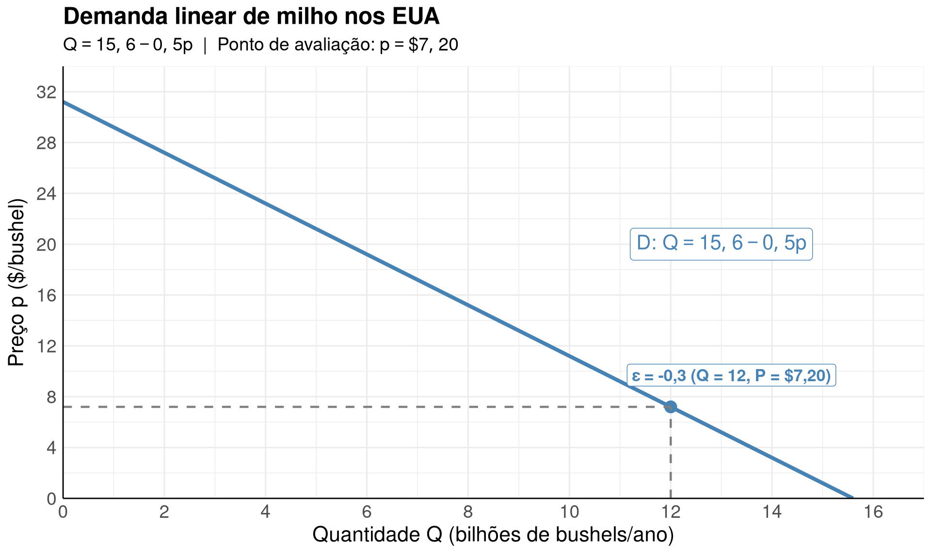
Perloff (2022), Problema Resolvido 2.2: A demanda linear de milho nos EUA é \(Q = 15{,}6 - 0{,}5p\) (bilhões de bushels/ano; preço em $/bushel). Calcule a elasticidade-preço da demanda no ponto \(p = \$7{,}20\).

Solução:

1. Calcule a quantidade no ponto de avaliação: \[Q = 15{,}6 - 0{,}5 \times 7{,}20 = 15{,}6 - 3{,}6 = 12 \text{ bilhões de bushels}\]

2. Aplique a fórmula da elasticidade-ponto: \[\varepsilon = -b \cdot \frac{p}{Q} = -0{,}5 \times \frac{7{,}20}{12} = -0{,}3\]

3. Interpretação: \(|\varepsilon| = 0{,}3 < 1\), portanto a demanda é inelástica. Um aumento de 1% no preço reduz a quantidade demandada em apenas 0,3%.

Implementação em R

suppressPackageStartupMessages({
  library(ggplot2)
  library(dplyr)
  library(latex2exp)
})

# Parâmetros da demanda: Q = 15.6 - 0.5*p  =>  p = 31.2 - 2*Q (convenção: P no eixo y)
a <- 15.6
b <- 0.5

# Curva de demanda: Q de 0 a 15.6
q_seq <- seq(0, 15.6, by = 0.1)
p_seq <- (a - q_seq) / b   # p = (a - Q) / b = 31.2 - 2*Q

dados_demanda <- data.frame(q = q_seq, p = p_seq)

# Ponto de avaliação
q0 <- 12
p0 <- 7.20
eps <- -b * (p0 / q0)  # -0.3

ggplot() +
  geom_line(
    data = dados_demanda,
    aes(x = q, y = p),
    color = "steelblue",
    linewidth = 1.4
  ) +
  geom_point(
    aes(x = q0, y = p0),
    color = "steelblue",
    size = 4
  ) +
  geom_segment(
    aes(x = q0, xend = q0, y = 0, yend = p0),
    linetype = "dashed", color = "gray50", linewidth = 0.8
  ) +
  geom_segment(
    aes(x = 0, xend = q0, y = p0, yend = p0),
    linetype = "dashed", color = "gray50", linewidth = 0.8
  ) +
  annotate(
    "label", x = q0 + 1.2, y = p0 + 2.5,
    label = "\u03B5 = -0,3 (Q = 12, P = $7,20)",
    fill = "white", label.size = 0.3,
    size = 4.5, color = "steelblue", fontface = "bold"
  ) +
  annotate(
    "label", x = 13, y = 20,
    label = TeX(r"(D: $Q = 15{,}6 - 0{,}5p$)"),
    fill = "white", label.size = 0.3,
    size = 5.5, color = "steelblue"
  ) +
  scale_x_continuous(
    breaks = seq(0, 16, by = 2),
    limits = c(0, 17),
    expand = c(0, 0)
  ) +
  scale_y_continuous(
    breaks = seq(0, 32, by = 4),
    limits = c(0, 34),
    expand = c(0, 0)
  ) +
  labs(
    title = "Demanda linear de milho nos EUA",
    subtitle = TeX(r"($Q = 15{,}6 - 0{,}5p$  |  Ponto de avaliação: $p = \$7{,}20$)"),
    x = TeX(r"(Quantidade $Q$ (bilhões de bushels/ano))"),
    y = TeX(r"(Preço $p$ (\$/bushel))")
  ) +
  theme_minimal() +
  theme(
    plot.title = element_text(size = 18, face = "bold"),
    plot.subtitle = element_text(size = 14),
    axis.line = element_line(color = "black", linewidth = 0.5),
    axis.title = element_text(size = 16, face = "bold"),
    axis.text = element_text(size = 14),
    legend.text = element_text(size = 13),
    legend.position = "bottom"
  )

Exercício Adicional

Exercício (Pindyck, 2013, Cap. 2): Considere a demanda de trigo nos EUA. Se o preço sobe de $4 para $5 por bushel e a quantidade cai de 15 para 12 bilhões de bushels, calcule a elasticidade-preço da demanda pelo método do ponto médio.

Interpretação

A elasticidade-preço calculada para o milho (\(\varepsilon = -0{,}3\)) indica que a demanda é inelástica: variações de preço têm efeitos proporcionalmente menores sobre a quantidade demandada. Esse resultado é típico de commodities agrícolas, pois o milho possui poucos substitutos próximos no curto prazo e faz parte de cadeias de consumo essenciais (alimentação, combustível). Produtores de bens com demanda inelástica têm maior poder de repasse de custos ao consumidor, pois aumentos de preço reduzem pouco a quantidade vendida e, portanto, a receita total aumenta com o preço.

Nota 2.2: Formas da função de demanda e elasticidade

Parte 1: demanda linear

Elasticidade varia ao longo da curva

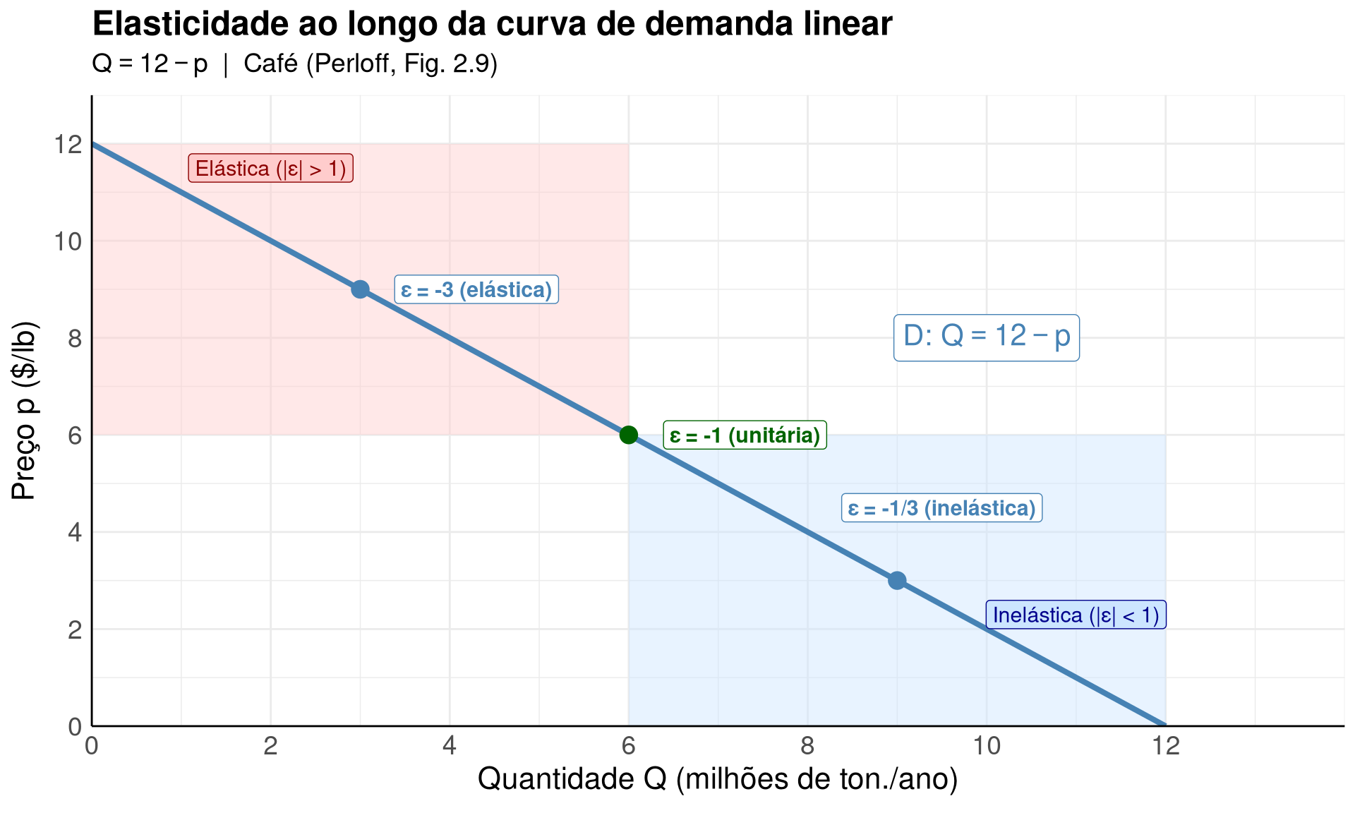
Em uma demanda linear \(Q = a - bp\), a elasticidade \(\varepsilon = -b \cdot p/Q\) varia ao longo da curva mesmo que a inclinação seja constante (Perloff, 2022):

• No intercepto horizontal (\(p = 0\), \(Q = a\)): \(\varepsilon = 0\) (perfeitamente inelástica)
• No ponto médio (\(p = a/(2b)\), \(Q = a/2\)): \(\varepsilon = -1\) (unitária)
• No intercepto vertical (\(Q = 0\), \(p = a/b\)): \(\varepsilon \to -\infty\) (perfeitamente elástica)

A intuição: mesmo que a inclinação \(-b\) seja constante, a razão \(p/Q\) varia. No topo da curva (preço elevado, quantidade baixa) a razão \(p/Q\) é alta, tornando a demanda elástica. Na base (preço baixo, quantidade alta) a razão é baixa, tornando a demanda inelástica.

Exemplo: demanda de café

Considere a demanda de café \(Q = 12 - p\) (milhões de toneladas/ano, preço em $/lb), baseada na Figura 2.9 de Perloff (2022). Aplicando a elasticidade-ponto:

\[\varepsilon = \frac{dQ}{dp} \cdot \frac{p}{Q} = (-1) \cdot \frac{p}{Q} = -\frac{p}{Q}\]

onde \(dQ/dp = -1\) é a derivada de \(Q = 12 - p\). Calculando em três pontos:

Preço (\(p\))	Quantidade (\(Q\))	\(\varepsilon = \frac{dQ}{dp} \cdot \frac{p}{Q} = (-1) \cdot \frac{p}{Q}\)	Classificação
3	9	\((-1) \times 3/9 = -1/3\)	Inelástica
6	6	\((-1) \times 6/6 = -1\)	Unitária
9	3	\((-1) \times 9/3 = -3\)	Elástica

Note que a mesma curva de demanda é inelástica na parte inferior e elástica na parte superior.

suppressPackageStartupMessages({
  library(ggplot2)
  library(dplyr)
  library(latex2exp)
})

# Demanda de café: Q = 12 - p  =>  p = 12 - Q (P no eixo y)
q_seq <- seq(0, 12, by = 0.1)
p_seq <- 12 - q_seq

dados <- data.frame(q = q_seq, p = p_seq)

# Pontos de avaliação
pts <- data.frame(
  q   = c(9, 6, 3),
  p   = c(3, 6, 9),
  eps = c(-1/3, -1, -3),
  lab = c("ε = −1/3\n(inelástica)", "ε = −1\n(unitária)", "ε = −3\n(elástica)")
)

ggplot() +
  # Região inelástica (p < 6)
  annotate("rect",
    xmin = 6, xmax = 12, ymin = 0, ymax = 6,
    fill = "#cce5ff", alpha = 0.45
  ) +
  # Região elástica (p > 6)
  annotate("rect",
    xmin = 0, xmax = 6, ymin = 6, ymax = 12,
    fill = "#ffcccc", alpha = 0.45
  ) +
  # Curva de demanda
  geom_line(
    data = dados,
    aes(x = q, y = p),
    color = "steelblue",
    linewidth = 1.4
  ) +
  # Pontos marcados
  geom_point(
    data = pts,
    aes(x = q, y = p),
    color = c("steelblue", "darkgreen", "steelblue"),
    size = 4
  ) +
  # Rótulos de elasticidade
  annotate("label", x = 9 + 0.5, y = 4.5,
    label = "\u03B5 = -1/3 (inel\u00E1stica)",
    fill = "white", label.size = 0.3,
    size = 4, color = "steelblue", fontface = "bold"
  ) +
  annotate("label", x = 6 + 1.3, y = 6,
    label = "\u03B5 = -1 (unit\u00E1ria)",
    fill = "white", label.size = 0.3,
    size = 4, color = "darkgreen", fontface = "bold"
  ) +
  annotate("label", x = 3 + 1.3, y = 9,
    label = "\u03B5 = -3 (el\u00E1stica)",
    fill = "white", label.size = 0.3,
    size = 4, color = "steelblue", fontface = "bold"
  ) +
  # Anotações de regiões
  annotate("label", x = 2, y = 11.5,
    label = "El\u00E1stica (|\u03B5| > 1)",
    fill = "#ffcccc", label.size = 0.3,
    size = 4, color = "darkred"
  ) +
  annotate("label", x = 11, y = 2.3,
    label = "Inel\u00E1stica (|\u03B5| < 1)",
    fill = "#cce5ff", label.size = 0.3,
    size = 4, color = "darkblue"
  ) +
  annotate("label", x = 10, y = 8,
    label = TeX(r"(D: $Q = 12 - p$)"),
    fill = "white", label.size = 0.3,
    size = 5.5, color = "steelblue"
  ) +
  scale_x_continuous(
    breaks = seq(0, 12, by = 2),
    limits = c(0, 14),
    expand = c(0, 0)
  ) +
  scale_y_continuous(
    breaks = seq(0, 12, by = 2),
    limits = c(0, 13),
    expand = c(0, 0)
  ) +
  labs(
    title = "Elasticidade ao longo da curva de demanda linear",
    subtitle = TeX(r"($Q = 12 - p$  |  Café (Perloff, Fig. 2.9))"),
    x = TeX(r"(Quantidade $Q$ (milhões de ton./ano))"),
    y = TeX(r"(Preço $p$ (\$/lb))")
  ) +
  theme_minimal() +
  theme(
    axis.line = element_line(color = "black", linewidth = 0.5),
    plot.title = element_text(size = 18, face = "bold"),
    plot.subtitle = element_text(size = 14),
    axis.title = element_text(size = 16, face = "bold"),
    axis.text = element_text(size = 14),
    legend.text = element_text(size = 13),
    legend.position = "bottom"
  )

Parte 2: demanda com elasticidade constante

A elasticidade varia ao longo da maioria das curvas de demanda, não apenas das lineares. Porém, existe uma classe especial de curvas em que a elasticidade é a mesma em todos os pontos (Perloff, 2022, pp. 57–58). Essas curvas têm a forma:

\[Q = Ap^\varepsilon\]

onde \(Q\) é a quantidade demandada, \(p\) é o preço, \(A > 0\) é uma constante de escala e \(\varepsilon < 0\) é a elasticidade-preço (constante ao longo de toda a curva).

Exemplo: a demanda estimada para apps na Apple Store é \(Q = 1{,}4p^{-2}\), onde \(A = 1{,}4\) (a quantidade seria 1,4 milhão de apps se o preço fosse $1) e \(\varepsilon = -2\) (Ghose e Han, 2014, conforme citado em Perloff). Um aumento de 1% no preço sempre reduz a demanda em 2%, independentemente do nível de preço.

Prova de que a elasticidade é constante

Queremos mostrar que, para \(Q = Ap^\varepsilon\), a elasticidade é igual a \(\varepsilon\) em qualquer ponto da curva. Usamos a definição \(E = \frac{dQ}{dp} \cdot \frac{p}{Q}\) e calculamos cada termo.

Passo 1: derivar \(Q = Ap^\varepsilon\) em relação a \(p\).

A constante \(A\) permanece e aplicamos a regra da potência ao termo \(p^\varepsilon\) (derivada de \(p^n\) é \(n \cdot p^{n-1}\)):

\[\frac{dQ}{dp} = A \cdot \varepsilon \cdot p^{\varepsilon - 1} = \varepsilon A p^{\varepsilon - 1}\]

Passo 2: montar a fórmula da elasticidade.

Substituímos \(dQ/dp\) e \(Q = Ap^\varepsilon\) na definição:

\[E = \underbrace{\varepsilon A p^{\varepsilon - 1}}_{\text{derivada}} \cdot \frac{p}{\underbrace{Ap^\varepsilon}_{Q}}\]

Passo 3: cancelar \(A\).

O fator \(A\) aparece no numerador (da derivada) e no denominador (de \(Q\)):

\[E = \varepsilon \cdot \frac{\cancel{A}}{\cancel{A}} \cdot \frac{p^{\varepsilon - 1} \cdot p}{p^\varepsilon}\]

Passo 4: simplificar as potências de \(p\).

No numerador, \(p^{\varepsilon - 1} \cdot p = p^{(\varepsilon - 1) + 1} = p^\varepsilon\). No denominador, temos \(p^\varepsilon\):

\[E = \varepsilon \cdot \frac{p^\varepsilon}{p^\varepsilon} = \varepsilon \cdot 1 = \varepsilon\]

Como o resultado final é simplesmente \(\varepsilon\), sem nenhum \(p\) ou \(Q\), a elasticidade é a mesma em qualquer ponto da curva.

Verificação numérica com o exemplo dos apps.

Vamos conferir usando \(Q = 1{,}4p^{-2}\) no ponto \(p = 2\):

Quantidade: substituindo \(p = 2\) na função de demanda:

\[Q = 1{,}4 \times 2^{-2} = 1{,}4 \times \frac{1}{4} = 0{,}35\]

Derivada: aplicando a regra da potência a \(Q = 1{,}4 \cdot p^{-2}\):

\[\frac{dQ}{dp} = 1{,}4 \times (-2) \times p^{-3} = -2{,}8 \times p^{-3}\]

Avaliando em \(p = 2\):

\[\frac{dQ}{dp}\bigg|_{p=2} = -2{,}8 \times 2^{-3} = -2{,}8 \times \frac{1}{8} = -0{,}35\]

Elasticidade: substituindo na definição \(E = \frac{dQ}{dp} \cdot \frac{p}{Q}\):

\[E = (-0{,}35) \times \frac{2}{0{,}35} = (-0{,}35) \times 5{,}714 = -2{,}0 = \varepsilon \quad \checkmark\]

O resultado confirma: a elasticidade é exatamente \(-2\) (o expoente da função), independentemente do ponto escolhido.

Parte 3: logaritmos e formas funcionais

Por que a economia usa logaritmos?

O uso de logaritmos em modelos econômicos tem uma razão prática: para variações pequenas, \(\Delta \ln X \approx \Delta X / X\), ou seja, a variação do logaritmo aproxima a variação percentual (Wooldridge, 2020, cap. 2 e 6). Dependendo de quais variáveis estão em log, a interpretação do coeficiente \(\beta_1\) muda:

Especificação	Equação	Interpretação de \(\beta_1\)
Lin-lin	\(Q = \beta_0 + \beta_1 p\)	\(\Delta p = 1\) unidade \(\Rightarrow\) \(\Delta Q = \beta_1\) unidades
Log-log	\(\ln Q = \beta_0 + \beta_1 \ln p\)	\(\uparrow 1\%\) em \(p\) \(\Rightarrow\) \(\Delta Q = \beta_1\%\) (elasticidade)
Log-lin	\(\ln Q = \beta_0 + \beta_1 p\)	\(\Delta p = 1\) unidade \(\Rightarrow\) \(\Delta Q = \beta_1 \times 100\%\)
Lin-log	\(Q = \beta_0 + \beta_1 \ln p\)	\(\uparrow 1\%\) em \(p\) \(\Rightarrow\) \(\Delta Q = \beta_1 / 100\) unidades

A especificação log-log é a mais usada em microeconomia porque \(\beta_1\) é diretamente a elasticidade, sem transformações.

Calculando a elasticidade em cada especificação

Aplicando a definição \(E = \frac{dQ}{dp} \cdot \frac{p}{Q}\) a cada caso:

Lin-lin: \(Q = \beta_0 + \beta_1 p\)

A derivada é \(dQ/dp = \beta_1\). A elasticidade varia conforme o ponto:

\[E = \beta_1 \cdot \frac{p}{Q} = \beta_1 \cdot \frac{p}{\beta_0 + \beta_1 p}\]

Log-log: \(\ln Q = \beta_0 + \beta_1 \ln p\)

Derivando ambos os lados em relação a \(p\): \(\frac{1}{Q} \cdot \frac{dQ}{dp} = \beta_1 \cdot \frac{1}{p}\), logo \(\frac{dQ}{dp} = \beta_1 \cdot \frac{Q}{p}\). Substituindo:

\[E = \beta_1 \cdot \frac{Q}{p} \cdot \frac{p}{Q} = \beta_1\]

A elasticidade é constante em todos os pontos.

Log-lin: \(\ln Q = \beta_0 + \beta_1 p\)

Derivando: \(\frac{1}{Q} \cdot \frac{dQ}{dp} = \beta_1\), logo \(\frac{dQ}{dp} = \beta_1 Q\). Substituindo:

\[E = \beta_1 Q \cdot \frac{p}{Q} = \beta_1 p\]

A elasticidade depende do nível de preço.

Lin-log: \(Q = \beta_0 + \beta_1 \ln p\)

Derivando: \(\frac{dQ}{dp} = \frac{\beta_1}{p}\). Substituindo:

\[E = \frac{\beta_1}{p} \cdot \frac{p}{Q} = \frac{\beta_1}{Q}\]

A elasticidade depende do nível de quantidade.

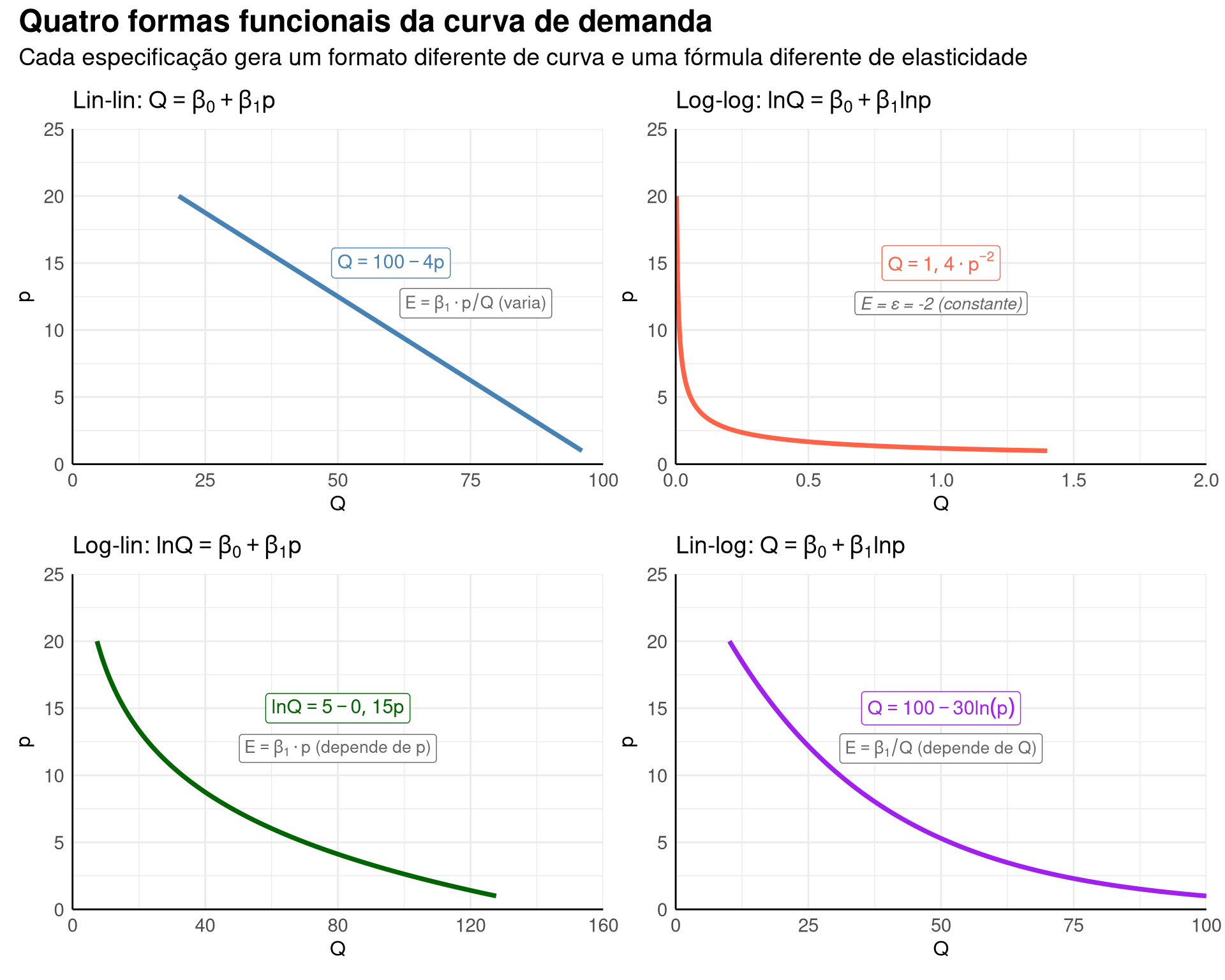
Resumo: apenas a especificação log-log produz elasticidade constante. Nas outras três, a elasticidade varia conforme o ponto na curva.

Formato das curvas de demanda

suppressPackageStartupMessages({
  library(ggplot2)
  library(patchwork)
  library(latex2exp)
})

# Tema comum
tema <- theme_minimal() +
  theme(
    plot.title = element_text(size = 14, face = "bold"),
    plot.subtitle = element_text(size = 11),
    axis.line = element_line(color = "black", linewidth = 0.5),
    axis.title = element_text(size = 12, face = "bold"),
    axis.text = element_text(size = 11)
  )

p_seq <- seq(1, 20, length.out = 300)

# 1. Lin-lin: Q = 100 - 4p
q_linlin <- 100 - 4 * p_seq
d_linlin <- data.frame(p = p_seq, q = q_linlin)
d_linlin <- d_linlin[d_linlin$q > 0, ]

p1 <- ggplot(d_linlin, aes(x = q, y = p)) +
  geom_line(color = "steelblue", linewidth = 1.3) +
  annotate("label", x = 60, y = 15,
    label = TeX(r"($Q = 100 - 4p$)"),
    fill = "white", label.size = 0.3,
    size = 4, color = "steelblue") +
  annotate("label", x = 76, y = 12,
    label = TeX(r"($E = \beta_1 \cdot p / Q$ (varia))"),
    fill = "white", label.size = 0.3,
    size = 3.5, color = "gray40", fontface = "italic") +
  scale_x_continuous(limits = c(0, 100), expand = c(0, 0)) +
  scale_y_continuous(limits = c(0, 25), expand = c(0, 0)) +
  labs(
    title = TeX(r"(Lin-lin: $Q = \beta_0 + \beta_1 p$)"),
    x = TeX(r"($Q$)"),
    y = TeX(r"($p$)")
  ) +
  tema

# 2. Log-log: Q = 1.4 * p^(-2)  =>  curva convexa
q_loglog <- 1.4 * p_seq^(-2)
d_loglog <- data.frame(p = p_seq, q = q_loglog)
d_loglog <- d_loglog[d_loglog$q <= 2, ]

p2 <- ggplot(d_loglog, aes(x = q, y = p)) +
  geom_line(color = "tomato", linewidth = 1.3) +
  annotate("label", x = 1.0, y = 15,
    label = TeX(r"($Q = 1{,}4 \cdot p^{-2}$)"),
    fill = "white", label.size = 0.3,
    size = 4, color = "tomato") +
  annotate("label", x = 1.0, y = 12,
    label = "E = \u03B5 = -2 (constante)",
    fill = "white", label.size = 0.3,
    size = 3.5, color = "gray40", fontface = "italic") +
  scale_x_continuous(limits = c(0, 2), expand = c(0, 0)) +
  scale_y_continuous(limits = c(0, 25), expand = c(0, 0)) +
  labs(
    title = TeX(r"(Log-log: $\ln Q = \beta_0 + \beta_1 \ln p$)"),
    x = TeX(r"($Q$)"),
    y = TeX(r"($p$)")
  ) +
  tema

# 3. Log-lin: ln Q = 5 - 0.15p  =>  Q = exp(5 - 0.15p)
q_loglin <- exp(5 - 0.15 * p_seq)
d_loglin <- data.frame(p = p_seq, q = q_loglin)

p3 <- ggplot(d_loglin, aes(x = q, y = p)) +
  geom_line(color = "darkgreen", linewidth = 1.3) +
  annotate("label", x = 80, y = 15,
    label = TeX(r"($\ln Q = 5 - 0{,}15p$)"),
    fill = "white", label.size = 0.3,
    size = 4, color = "darkgreen") +
  annotate("label", x = 80, y = 12,
    label = TeX(r"($E = \beta_1 \cdot p$ (depende de $p$))"),
    fill = "white", label.size = 0.3,
    size = 3.5, color = "gray40", fontface = "italic") +
  scale_x_continuous(limits = c(0, 160), expand = c(0, 0)) +
  scale_y_continuous(limits = c(0, 25), expand = c(0, 0)) +
  labs(
    title = TeX(r"(Log-lin: $\ln Q = \beta_0 + \beta_1 p$)"),
    x = TeX(r"($Q$)"),
    y = TeX(r"($p$)")
  ) +
  tema

# 4. Lin-log: Q = 100 - 30 ln(p)
q_linlog <- 100 - 30 * log(p_seq)
d_linlog <- data.frame(p = p_seq, q = q_linlog)
d_linlog <- d_linlog[d_linlog$q > 0, ]

p4 <- ggplot(d_linlog, aes(x = q, y = p)) +
  geom_line(color = "purple", linewidth = 1.3) +
  annotate("label", x = 50, y = 15,
    label = TeX(r"($Q = 100 - 30 \ln(p)$)"),
    fill = "white", label.size = 0.3,
    size = 4, color = "purple") +
  annotate("label", x = 50, y = 12,
    label = TeX(r"($E = \beta_1 / Q$ (depende de $Q$))"),
    fill = "white", label.size = 0.3,
    size = 3.5, color = "gray40", fontface = "italic") +
  scale_x_continuous(limits = c(0, 100), expand = c(0, 0)) +
  scale_y_continuous(limits = c(0, 25), expand = c(0, 0)) +
  labs(
    title = TeX(r"(Lin-log: $Q = \beta_0 + \beta_1 \ln p$)"),
    x = TeX(r"($Q$)"),
    y = TeX(r"($p$)")
  ) +
  tema

(p1 + p2) / (p3 + p4) +
  plot_annotation(
    title = "Quatro formas funcionais da curva de demanda",
    subtitle = "Cada especificação gera um formato diferente de curva e uma fórmula diferente de elasticidade",
    theme = theme(
      plot.title = element_text(size = 18, face = "bold"),
      plot.subtitle = element_text(size = 14)
    )
  )

Observe que cada especificação gera um formato diferente de curva: a lin-lin é uma reta, a log-log é uma hipérbole convexa, a log-lin decai exponencialmente e a lin-log tem formato logarítmico.

Quando usar cada especificação?

A escolha da forma funcional não é arbitrária. Ela reflete uma hipótese sobre como os agentes econômicos respondem a variações de preço: em termos absolutos ou percentuais? (Wooldridge, 2020, seção 6.2; Perloff, 2022, pp. 57–58)

Especificação	Hipótese sobre o comportamento	Quando faz sentido
Lin-lin	Uma variação absoluta fixa no preço (\(\Delta p = 1\)) causa sempre a mesma variação absoluta na quantidade	Relações aproximadamente lineares em faixas estreitas de preço. Exemplo: demanda local por um produto com preço regulado
Log-log	Uma variação percentual no preço (\(\uparrow 1\%\)) causa sempre a mesma variação percentual na quantidade	A maioria dos mercados. Agentes respondem a variações proporcionais: um aumento de 10% no preço importa igualmente se o preço é R$ 5 ou R$ 50. É a especificação padrão em microeconomia empírica
Log-lin	Uma variação absoluta fixa no preço causa sempre a mesma variação percentual na quantidade	Bens com tarifas reguladas ou preços administrados, onde a estrutura tarifária opera em valores absolutos. Exemplo: tarifa de água ou energia elétrica por faixa de consumo
Lin-log	Uma variação percentual no preço causa sempre a mesma variação absoluta na quantidade	Mercados onde o efeito do preço se esgota com o aumento da quantidade. Exemplo: gastos com publicidade (dobrar o investimento não dobra as vendas, apenas adiciona um número fixo de clientes)

A especificação log-log domina a literatura empírica em microeconomia porque a maioria das decisões econômicas responde a incentivos proporcionais, não absolutos. Um consumidor que reduz o consumo de gasolina em 5% quando o preço sobe 10% tende a manter essa proporção independentemente de o litro custar R$ 5 ou R$ 10.

Nota 2.3: Elasticidade e receita total

Desenvolvimento Teórico

A receita total é definida como \(R = p \cdot Q\). A questão central: quando uma firma altera seu preço, a receita sobe ou cai? A resposta depende da elasticidade da demanda (Nicholson e Snyder, 2018; Perloff, 2022).

Elasticidade	\(P \uparrow\)	\(P \downarrow\)
\(|\varepsilon| > 1\) (elástica)	\(RT \downarrow\)	\(RT \uparrow\)
\(|\varepsilon| = 1\) (unitária)	\(RT\) não muda	\(RT\) não muda
\(|\varepsilon| < 1\) (inelástica)	\(RT \uparrow\)	\(RT \downarrow\)

Formalização Matemática

Partindo de \(R = p \cdot Q(p)\), aplicamos a regra do produto:

\[\frac{dR}{dp} = Q + p \cdot \frac{dQ}{dp}\]

Fatorando \(Q\):

\[\frac{dR}{dp} = Q \left(1 + \frac{p}{Q} \cdot \frac{dQ}{dp}\right) = Q(1 + \varepsilon)\]

Análise dos três casos:

• Se \(|\varepsilon| > 1\) (elástica): \(\varepsilon < -1\), portanto \(1 + \varepsilon < 0\), logo \(dR/dp < 0\). Reduzir o preço aumenta a receita.
• Se \(|\varepsilon| < 1\) (inelástica): \(-1 < \varepsilon < 0\), portanto \(1 + \varepsilon > 0\), logo \(dR/dp > 0\). Elevar o preço aumenta a receita.
• Se \(|\varepsilon| = 1\) (unitária): \(\varepsilon = -1\), portanto \(1 + \varepsilon = 0\), logo \(dR/dp = 0\). A receita é máxima.

Exemplo Numérico

Uma firma de cimento com elasticidade-preço da demanda \(|E| = 2\) deseja prever sua receita diante de uma variação de 1% no preço do cimento.

Dados iniciais: a firma vende 10.000 toneladas de cimento ao preço de R$ 10 a tonelada. A receita é:

\[R = 10 \times 10.000 = \text{R\$} \; 100.000\]

Aumento de 1% no preço. Como \(|E| = 2\), a quantidade cai 2%:

\[\underbrace{(10 + 10 \times 0{,}01)}_{\text{novo preço}} \times \underbrace{(10.000 - 10.000 \times 0{,}02)}_{\text{nova quantidade}} = 10{,}10 \times 9.800 = \text{R\$} \; 98.980\]

A receita caiu de R$ 100.000 para R$ 98.980.

Redução de 1% no preço. A quantidade sobe 2%:

\[\underbrace{(10 - 10 \times 0{,}01)}_{\text{novo preço}} \times \underbrace{(10.000 + 10.000 \times 0{,}02)}_{\text{nova quantidade}} = 9{,}90 \times 10.200 = \text{R\$} \; 100.980\]

A receita subiu de R$ 100.000 para R$ 100.980.

Conclusão: como a demanda é elástica (\(|E| > 1\)), a queda na quantidade é proporcionalmente maior que o aumento no preço, e a firma aumenta sua receita reduzindo o preço.

Implementação em R

suppressPackageStartupMessages({
  library(ggplot2)
  library(dplyr)
  library(patchwork)
  library(latex2exp)
})

# Demanda linear: Q = 12 - p  =>  p = 12 - Q
# Receita total: R(p) = p * (12 - p) = 12p - p^2

q_seq <- seq(0, 12, by = 0.1)
p_seq <- 12 - q_seq  # p no eixo y

dados_d <- data.frame(q = q_seq, p = p_seq)

# Painel superior: curva de demanda com regiões
p_demand <- ggplot() +
  # Região inelástica (p < 6, q > 6)
  annotate("rect",
    xmin = 6, xmax = 12, ymin = 0, ymax = 6,
    fill = "#cce5ff", alpha = 0.45
  ) +
  # Região elástica (p > 6, q < 6)
  annotate("rect",
    xmin = 0, xmax = 6, ymin = 6, ymax = 12,
    fill = "#ffcccc", alpha = 0.45
  ) +
  geom_line(
    data = dados_d,
    aes(x = q, y = p),
    color = "steelblue",
    linewidth = 1.4
  ) +
  geom_point(aes(x = 6, y = 6), color = "darkgreen", size = 4) +
  geom_segment(
    aes(x = 6, xend = 6, y = 0, yend = 6),
    linetype = "dashed", color = "gray50", linewidth = 0.8
  ) +
  geom_segment(
    aes(x = 0, xend = 6, y = 6, yend = 6),
    linetype = "dashed", color = "gray50", linewidth = 0.8
  ) +
  annotate("label", x = 6 + 1.0, y = 7,
    label = "\u03B5 = -1 (ponto m\u00E9dio)",
    fill = "white", label.size = 0.3,
    size = 4, color = "darkgreen", fontface = "bold"
  ) +
  annotate("label", x = 3, y = 10.5,
    label = "El\u00E1stica (|\u03B5| > 1)",
    fill = "#ffcccc", label.size = 0.3,
    size = 4, color = "darkred"
  ) +
  annotate("label", x = 11, y = 3,
    label = "Inel\u00E1stica (|\u03B5| < 1)",
    fill = "#cce5ff", label.size = 0.3,
    size = 4, color = "darkblue"
  ) +
  annotate("label", x = 10.5, y = 8,
    label = TeX(r"(D: $Q = 12 - p$)"),
    fill = "white", label.size = 0.3,
    size = 5.5, color = "steelblue"
  ) +
  scale_x_continuous(
    breaks = seq(0, 12, by = 2),
    limits = c(0, 13),
    expand = c(0, 0)
  ) +
  scale_y_continuous(
    breaks = seq(0, 12, by = 2),
    limits = c(0, 13),
    expand = c(0, 0)
  ) +
  labs(
    title = TeX(r"(Curva de demanda: $Q = 12 - p$)"),
    x = TeX(r"(Quantidade ($Q$))"),
    y = TeX(r"(Preço ($p$))")
  ) +
  theme_minimal() +
  theme(
    plot.title = element_text(size = 18, face = "bold"),
    plot.subtitle = element_text(size = 14),
    axis.line = element_line(color = "black", linewidth = 0.5),
    axis.title = element_text(size = 16, face = "bold"),
    axis.text = element_text(size = 14),
    legend.text = element_text(size = 13),
    legend.position = "bottom"
  )

# Painel inferior: receita total R(p) = p*(12-p)
p_vals <- seq(0, 12, by = 0.1)
r_vals <- p_vals * (12 - p_vals)

dados_r <- data.frame(p = p_vals, r = r_vals)

p_revenue <- ggplot() +
  geom_line(
    data = dados_r,
    aes(x = p, y = r),
    color = "darkorange",
    linewidth = 1.4
  ) +
  geom_point(aes(x = 6, y = 36), color = "darkgreen", size = 4) +
  geom_segment(
    aes(x = 6, xend = 6, y = 0, yend = 36),
    linetype = "dashed", color = "gray50", linewidth = 0.8
  ) +
  annotate("label", x = 6 + 1.5, y = 36,
    label = "RT m\u00E1x = 36 (p = 6, \u03B5 = -1)",
    fill = "white", label.size = 0.3,
    size = 4, color = "darkgreen", fontface = "bold"
  ) +
  annotate("label", x = 1.5, y = 23,
    label = "RT sobe\ncom p\n(inelástica)",
    fill = "#cce5ff", label.size = 0.3,
    size = 3.8, color = "darkblue"
  ) +
  annotate("label", x = 10.5, y = 23,
    label = "RT cai\ncom p\n(elástica)",
    fill = "#ffcccc", label.size = 0.3,
    size = 3.8, color = "darkred"
  ) +
  scale_x_continuous(
    breaks = seq(0, 12, by = 2),
    limits = c(0, 13),
    expand = c(0, 0)
  ) +
  scale_y_continuous(
    breaks = seq(0, 36, by = 6),
    limits = c(0, 40),
    expand = c(0, 0)
  ) +
  labs(
    title = TeX(r"(Receita total: $R(p) = p \cdot (12 - p)$)"),
    x = TeX(r"(Preço ($p$))"),
    y = TeX(r"(Receita total ($R$))")
  ) +
  theme_minimal() +
  theme(
    plot.title = element_text(size = 18, face = "bold"),
    plot.subtitle = element_text(size = 14),
    axis.line = element_line(color = "black", linewidth = 0.5),
    axis.title = element_text(size = 16, face = "bold"),
    axis.text = element_text(size = 14),
    legend.text = element_text(size = 13),
    legend.position = "bottom"
  )

p_demand / p_revenue

Exercício Adicional

Exercício (Bergstrom e Varian, 2009, cap. 15): Considere a função de demanda \(Q = 100/p^2\).

1. Calcule a elasticidade-preço.

2. Calcule a receita total como função de \(p\).

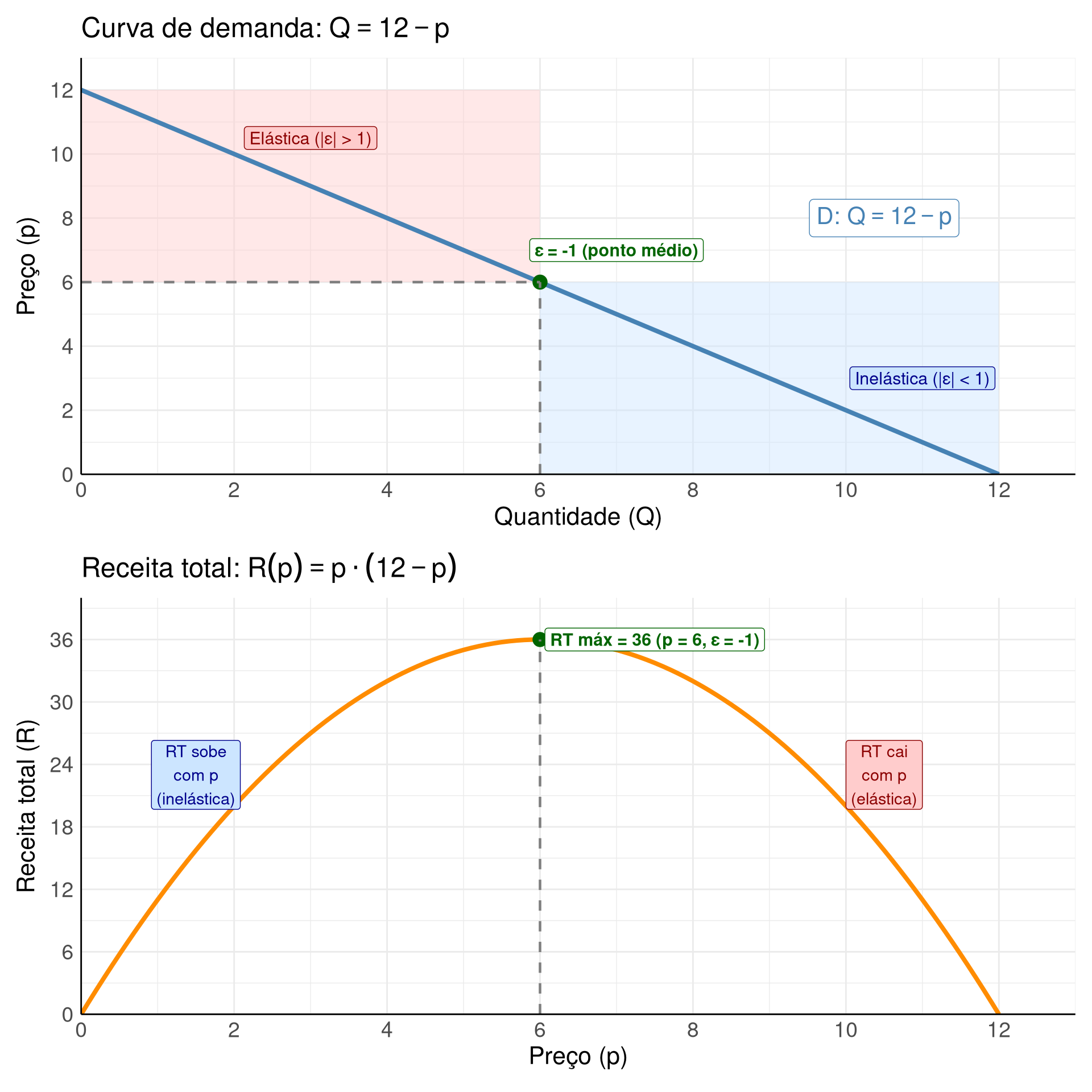
3. A receita total é constante, crescente ou decrescente em \(p\)? Explique usando a relação \(dR/dp = Q(1 + \varepsilon)\).

Interpretação

O gráfico duplo revela a conexão íntima entre elasticidade e receita. A receita atinge seu pico exatamente no ponto de elasticidade unitária, o “ponto ideal” para a firma. Na porção elástica, reduzir o preço atrai clientes proporcionalmente mais, elevando a receita. Na porção inelástica, elevar o preço perde clientes proporcionalmente menos, também elevando a receita. Esse resultado é fundamental para a estratégia de precificação.

Nota 2.4: Elasticidade-renda e elasticidade-preço cruzada

Desenvolvimento Teórico: elasticidade-renda

A elasticidade-renda da demanda mede a variação percentual na quantidade demandada em resposta a uma variação percentual na renda. Formalmente (Perloff, 2022):

\[E_R^D = \frac{\partial Q}{\partial Y} \cdot \frac{Y}{Q}\]

Classificação	Condição	Exemplos
Bem normal	\(E_R^D > 0\)	A maioria dos bens
Bem inferior	\(E_R^D < 0\)	Transporte público (para alta renda)
Bem de luxo	\(E_R^D > 1\)	Viagens internacionais, automóveis
Bem de necessidade	\(0 < E_R^D < 1\)	Alimentos, acesso à internet

Lei de Engel: à medida que a renda aumenta, a proporção gasta com alimentos diminui (a elasticidade-renda de alimentos é positiva, mas menor que 1).

Desenvolvimento Teórico: elasticidade cruzada

A elasticidade-preço cruzada mede como a quantidade demandada de um bem \(X\) responde ao preço de outro bem \(Y\):

\[E_{XY}^D = \frac{\partial Q_X}{\partial p_Y} \cdot \frac{p_Y}{Q_X}\]

Sinal	Relação	Exemplo
\(E_{XY}^D > 0\)	Substitutos	Coca-Cola e Pepsi
\(E_{XY}^D < 0\)	Complementares	Café e açúcar
\(E_{XY}^D = 0\)	Independentes	Sapatos e arroz

Exercício Resolvido

Problema (Perloff, 2022, pp. 59–60): a função de demanda estimada para o café é:

\[Q = 8{,}5 - p - 0{,}3p_s + 0{,}1Y\]

onde \(Q\) é a quantidade demandada (milhões de toneladas/ano), \(p\) é o preço do café ($/lb), \(p_s\) é o preço do açúcar ($/lb) e \(Y\) é a renda (milhares de dólares). No equilíbrio, \(Q = 10\), \(p_s = \$0{,}20\)/lb e \(Y = 35\).

Calcule a elasticidade-renda e a elasticidade cruzada café-açúcar. Classifique os bens.

Elasticidade-renda:

A derivada parcial de \(Q\) em relação a \(Y\) é \(\frac{\partial Q}{\partial Y} = 0{,}1\). Substituindo na fórmula:

\[E_R^D = \frac{\partial Q}{\partial Y} \cdot \frac{Y}{Q} = 0{,}1 \times \frac{35}{10} = 0{,}35\]

Como \(E_R^D = 0{,}35 > 0\), o café é um bem normal (a demanda cresce com a renda). Como \(E_R^D < 1\), é classificado como necessidade: um aumento de 10% na renda eleva a demanda por café em apenas 3,5%.

Elasticidade cruzada café-açúcar:

A derivada parcial de \(Q\) em relação a \(p_s\) é \(\frac{\partial Q}{\partial p_s} = -0{,}3\). Substituindo:

\[E_{XY}^D = \frac{\partial Q}{\partial p_s} \cdot \frac{p_s}{Q} = -0{,}3 \times \frac{0{,}20}{10} = -0{,}006\]

Como \(E_{XY}^D < 0\), café e açúcar são complementares: um aumento no preço do açúcar reduz a demanda por café. Porém, o efeito é muito fraco: um aumento de 1% no preço do açúcar reduz a demanda por café em apenas 0,006%.

Exercício Adicional

Exercício (Pindyck e Rubinfeld, 2013, cap. 2): Um estudo estimou que a elasticidade-renda da demanda por refeições em restaurantes é 1,4 e por alimentos consumidos em casa é 0,4. (a) Classifique cada bem. (b) Se a renda aumenta 10%, qual o efeito sobre a quantidade demandada de cada um? (c) Como a Lei de Engel se manifesta neste exemplo?

Interpretação

As elasticidades-renda e cruzada revelam como os bens se relacionam entre si e com a renda. O exemplo do café mostra que, embora café e açúcar sejam complementares, o efeito cruzado é ínfimo: um aumento de 1% no preço do açúcar reduz a demanda por café em apenas 0,006%. As elasticidades-renda são cruciais para prever o crescimento da demanda à medida que as economias se desenvolvem: bens de luxo crescem mais rapidamente do que necessidades.

Nota 2.5: Elasticidade-preço da oferta e horizonte temporal

Desenvolvimento Teórico

A elasticidade-preço da oferta mede a variação percentual na quantidade ofertada em resposta a uma variação percentual no preço:

\[E_P^S = \frac{\partial Q}{\partial p} \cdot \frac{p}{Q}\]

(Perloff, 2022)

Em geral, \(E_P^S > 0\) (lei da oferta). A classificação é análoga à da demanda: perfeitamente inelástica (\(E_P^S = 0\)), inelástica (\(0 < E_P^S < 1\)), unitária (\(E_P^S = 1\)), elástica (\(E_P^S > 1\)) e perfeitamente elástica (\(E_P^S \to \infty\)).

Resultado especial (Perloff, 2022, Problema Resolvido 2.4): qualquer oferta linear que passe pela origem tem a forma \(Q = Bp\) (com \(B > 0\)). Nesse caso, a elasticidade é unitária em todos os pontos, pois:

\[E_P^S = \frac{dQ}{dp} \cdot \frac{p}{Q} = B \cdot \frac{p}{Bp} = 1\]

O \(B\) cancela, e a elasticidade não depende do ponto na curva.

Intuição econômica: quando a oferta passa pela origem, ao preço zero ninguém produz (\(Q = 0\)). A partir daí, cada aumento percentual no preço gera exatamente o mesmo aumento percentual na quantidade ofertada. Por exemplo, se \(Q = 2p\): ao preço 5 a oferta é 10, ao preço 10 a oferta é 20. O preço dobrou e a quantidade também dobrou. Isso vale em qualquer ponto da curva porque não há um “piso” de produção (intercepto) que distorça a proporção.

Quando a oferta tem intercepto positivo (\(Q = a + Bp\), com \(a > 0\)), parte da produção existe mesmo a preço zero, o que faz a elasticidade ser menor que 1. Quando tem intercepto negativo (\(a < 0\)), há um preço mínimo para começar a produzir, e a elasticidade é maior que 1.

Curto prazo vs. longo prazo

As elasticidades diferem conforme o horizonte temporal.

Demanda:

• Curto prazo: mais inelástica (poucos substitutos imediatos)
• Longo prazo: mais elástica (consumidores encontram substitutos e mudam hábitos)
• Exemplo: gasolina. No curto prazo \(E_P^D = -0{,}16\); no longo prazo \(E_P^D = -0{,}43\) (Liddle, 2012, conforme citado em Perloff, p. 62)

Oferta:

• Curto prazo: mais inelástica (capacidade fixa)
• Longo prazo: mais elástica (firmas expandem e novos entrantes surgem)
• Exemplo: elasticidade da oferta de serviços de saúde é 0,7 no curto prazo e 1,4 no longo prazo (Clemens e Gottlieb, 2014, conforme citado em Perloff)

Exercício Resolvido

Problema (Perloff, 2022, Equação 2.27): a função de oferta estimada para o milho nos EUA é:

\[Q = 10{,}2 + 0{,}25p\]

onde \(Q\) é a quantidade ofertada (bilhões de bushels/ano) e \(p\) é o preço (dólares/bushel). Calcule a elasticidade-preço da oferta no ponto \(p = \$7{,}20\).

Passo 1: calcular a quantidade ofertada.

\[Q = 10{,}2 + 0{,}25 \times 7{,}20 = 10{,}2 + 1{,}8 = 12 \text{ bilhões de bushels}\]

Passo 2: identificar a derivada. Como \(Q = 10{,}2 + 0{,}25p\), temos \(dQ/dp = 0{,}25\).

Passo 3: calcular a elasticidade.

\[E_P^S = \frac{dQ}{dp} \cdot \frac{p}{Q} = 0{,}25 \times \frac{7{,}20}{12} = 0{,}15\]

A oferta é inelástica (\(E_P^S < 1\)): um aumento de 1% no preço eleva a quantidade ofertada em apenas 0,15%.

Comparação com a demanda: no Note 2.1 calculamos a elasticidade-preço da demanda de milho como \(E_P^D = -0{,}3\). Ambas são inelásticas, mas a demanda é mais responsiva do que a oferta (\(|-0{,}3| > 0{,}15\)). Note que a oferta tem intercepto positivo (\(a = 10{,}2 > 0\)), o que significa que mesmo a preço zero haveria produção de milho, confirmando a elasticidade menor que 1 discutida acima.

Exercício Adicional

Exercício (Nicholson e Snyder, 2018, cap. 12): Mostre que a função de oferta \(Q = Bp^{E_P^S}\) com \(E_P^S = 1\) é linear e passa pela origem. (Dica: se \(E_P^S = 1\), então \(Q = Bp^1 = Bp\), que é uma reta com inclinação \(B\) passando pelo ponto \((0, 0)\).)

Interpretação

A comparação entre as elasticidades de curto e longo prazo tem implicações relevantes para a política econômica. Choques de oferta (como embargos de petróleo ou quebras de safra) causam elevações de preço maiores no curto prazo precisamente porque tanto a demanda quanto a oferta são mais inelásticas. Com o tempo, consumidores encontram substitutos e produtores ajustam a capacidade, amortecendo o efeito sobre o preço. Isso explica por que a volatilidade dos preços de commodities tende a ser mais intensa para choques de curta duração.

Nota 2.6: Aplicação: demanda de água no Nordeste brasileiro

Contexto

O setor de saneamento básico no Brasil opera sob regime de monopólio natural. Para determinar tarifas que maximizem o bem-estar social, é necessário estimar a elasticidade-preço da demanda de água. Melo e Jorge Neto (2010) estimaram a função de demanda residencial de água para a região Nordeste, utilizando dados do Banco do Nordeste (BNB, 1997) para municípios da região.

A função de demanda estimada

Os autores estimaram a seguinte função log-linear por mínimos quadrados ordinários:

\[\ln Q = 0{,}491 - 0{,}550 \ln P + 0{,}239 \ln R + 0{,}080 \ln N + 0{,}018 \ln T + 0{,}269 D_e\]

onde:

• \(Q\) = consumo de água (m³/família/mês)
• \(P\) = preço marginal da água (R$/m³)
• \(R\) = renda do domicílio (R$/mês)
• \(N\) = número de cômodos (proxy para tamanho da família ou riqueza)
• \(T\) = tempo de moradia no domicílio (anos)
• \(D_e\) = variável dummy para esgoto (1 se o domicílio está conectado à rede de esgoto, 0 caso contrário)

Interpretação dos coeficientes

Como a equação está na forma log-linear (\(\ln Q = \beta_0 + \beta_1 \ln P + \ldots\)), os coeficientes são diretamente as elasticidades:

• Elasticidade-preço: \(E_P^D = -0{,}550\). A demanda é inelástica (\(|E_P^D| < 1\)): um aumento de 1% no preço da água reduz o consumo em 0,55%. Isso é esperado para um bem essencial com poucos substitutos.
• Elasticidade-renda: \(E_R^D = 0{,}239\). A água é um bem normal (\(E_R^D > 0\)) classificado como necessidade (\(E_R^D < 1\)): um aumento de 1% na renda eleva o consumo em apenas 0,24%.
• Cômodos: um aumento de 1% no número de cômodos eleva o consumo em 0,08%.
• Tempo de moradia: efeito pequeno (0,018%).
• Esgoto: domicílios conectados à rede de esgoto consomem mais água, pois não sofrem restrição de escoamento.

Redução à demanda em função do preço

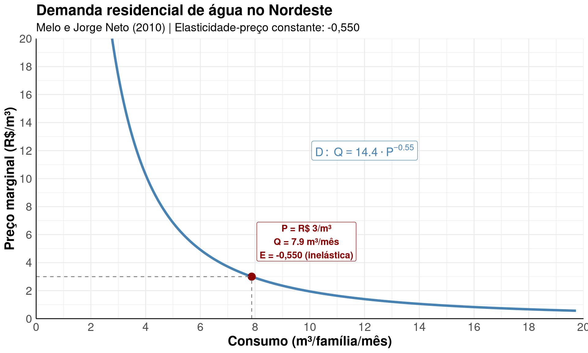
Para obter uma curva de demanda apenas em função do preço, os autores substituíram os valores médios das demais variáveis (\(R = 307{,}96\); \(N = 4{,}47\); \(T = 10{,}13\); \(D_e = 0{,}39\)):

\[\ln Q = 0{,}491 + 0{,}239 \ln(307{,}96) + 0{,}080 \ln(4{,}47) + 0{,}018 \ln(10{,}13) + 0{,}269 \times 0{,}39 - 0{,}550 \ln P\]

Calculando os termos constantes:

• \(0{,}239 \times \ln(307{,}96) = 0{,}239 \times 5{,}730 = 1{,}370\)
• \(0{,}080 \times \ln(4{,}47) = 0{,}080 \times 1{,}497 = 0{,}120\)
• \(0{,}018 \times \ln(10{,}13) = 0{,}018 \times 2{,}316 = 0{,}042\)
• \(0{,}269 \times 0{,}39 = 0{,}105\)

Somando: \(0{,}491 + 1{,}370 + 0{,}120 + 0{,}042 + 0{,}105 = 2{,}128\)

A função reduzida fica:

\[\boxed{\ln Q = 2{,}668 - 0{,}550 \ln P}\]

Que na forma exponencial equivale a \(Q = e^{2{,}668} \cdot P^{-0{,}550} \approx 14{,}41 \cdot P^{-0{,}550}\). Esta é uma demanda com elasticidade constante (como estudado no Callout 2), com \(\varepsilon = -0{,}550\) em todos os pontos da curva.

Implementação em R

suppressPackageStartupMessages({
  library(ggplot2)
})

# Função de demanda reduzida: ln Q = 2.668 - 0.550 ln P
# Q = exp(2.668) * P^(-0.550)
A <- exp(2.668)
eps <- -0.550

p_seq <- seq(0.5, 20, length.out = 300)
q_seq <- A * p_seq^eps

dados <- data.frame(p = p_seq, q = q_seq)

# Ponto de referência: preço médio ~ R$ 3/m³
p_ref <- 3
q_ref <- A * p_ref^eps

ggplot() +
  geom_line(
    data = dados,
    aes(x = q, y = p),
    color = "steelblue",
    linewidth = 1.4
  ) +
  geom_point(
    aes(x = q_ref, y = p_ref),
    color = "darkred", size = 4
  ) +
  geom_segment(
    aes(x = q_ref, xend = q_ref, y = 0, yend = p_ref),
    linetype = "dashed", color = "gray50"
  ) +
  geom_segment(
    aes(x = 0, xend = q_ref, y = p_ref, yend = p_ref),
    linetype = "dashed", color = "gray50"
  ) +
  annotate(
    "label", x = q_ref + 2, y = p_ref + 2.5,
    label = paste0(
      "P = R$ ", p_ref, "/m³\n",
      "Q = ", round(q_ref, 1), " m³/mês\n",
      "E = -0,550 (inelástica)"
    ),
    fill = "white", label.size = 0.3,
    size = 4, color = "darkred", fontface = "bold"
  ) +
  annotate(
    "label", x = 12, y = 12,
    label = "D:~Q == 14.4 %.% P^{-0.55}",
    parse = TRUE,
    fill = "white", label.size = 0.3,
    size = 5, color = "steelblue"
  ) +
  scale_x_continuous(
    breaks = seq(0, 20, by = 2),
    limits = c(0, 20),
    expand = c(0, 0)
  ) +
  scale_y_continuous(
    breaks = seq(0, 20, by = 2),
    limits = c(0, 20),
    expand = c(0, 0)
  ) +
  labs(
    title = "Demanda residencial de água no Nordeste",
    subtitle = "Melo e Jorge Neto (2010) | Elasticidade-preço constante: -0,550",
    x = "Consumo (m³/família/mês)",
    y = "Preço marginal (R$/m³)"
  ) +
  theme_minimal() +
  theme(
    plot.title = element_text(size = 18, face = "bold"),
    plot.subtitle = element_text(size = 14),
    axis.line = element_line(color = "black", linewidth = 0.5),
    axis.title = element_text(size = 16, face = "bold"),
    axis.text = element_text(size = 14),
    legend.text = element_text(size = 13),
    legend.position = "bottom"
  )

Interpretação

Este exemplo ilustra vários conceitos discutidos nos callouts anteriores:

1. Forma log-linear e elasticidade constante: a equação estimada está na forma \(\ln Q = \ln A + \varepsilon \ln P\), que corresponde a \(Q = AP^\varepsilon\) (ver Note 2.2). O coeficiente de \(\ln P\) é diretamente a elasticidade-preço.

2. Demanda inelástica para bens essenciais: com \(E_P^D = -0{,}550\), a água se comporta como esperado para um bem essencial, com poucos substitutos no curto prazo. Mesmo aumentos significativos no preço reduzem o consumo proporcionalmente menos.

3. Elasticidade-renda como necessidade: \(E_R^D = 0{,}239 < 1\) confirma a Lei de Engel (ver Note 2.4): à medida que a renda cresce, a proporção gasta com água diminui.

4. Implicação para política tarifária: como a demanda é inelástica, aumentos de tarifa elevam a receita das companhias de saneamento (ver Note 2.3), mas reduzem pouco o consumo. Isso é relevante para o debate sobre regulação de preços no setor.

Referências

BERGSTROM, T. C.; VARIAN, H. R. Workouts in Intermediate Microeconomics: For Intermediate Microeconomics and Intermediate Microeconomics with Calculus. 8th. ed. New York: W. W. Norton & Company, 2009.

MELO, J. A. M. DE; JORGE NETO, P. DE M. Bem-estar social, regulação e eficiência no setor de saneamento básico. Revista Econômica do Nordeste, v. 41, n. 4, p. 763–780, 2010.

NICHOLSON, W.; SNYDER, C. Teoria microeconômica: princı́pios básicos e aplicações. [s.l.] Cengage Learning Edições, 2018.

PERLOFF, J. M. Microeconomics with Calculus, Global Edition. 5. ed. [s.l.] Pearson, 2022.

PINDYCK, R. S.; RUBINFELD, D. L. Microeconomia. [s.l.] Pearson Education do Brasil, 2013.

WOOLDRIDGE, J. M. Introductory Econometrics: A Modern Approach. 7th. ed. Boston: Cengage Learning, 2020.