4 Lattes Projects
rio::import('rawfiles/projetos.rds') |>
    tibble::tibble() ->
    projetos

# rio::export(projetos, 'rawfiles/projetos.xlsx')

projetos |>
    dplyr::group_by(natureza, situacao) |>
    tally(name = 'quantidade') |>
        datatable(
        extensions = 'Buttons',
        rownames = F,
        options = list(
                    dom = 'Bfrtip',
                    pageLength = 12,
                    buttons = list(list(
                                        extend = 'collection',
                                        buttons = list(list(extend = 'csv', filename = 'data'),
                                                        list(extend = 'excel', filename = 'data')),
                                                        text = 'Download'))))
projetos |>
dplyr::filter(natureza == 'PESQUISA') ->
pesq
pesq |>
dplyr::mutate(texto = paste(nome_do_projeto, descricao_do_projeto, sep = '. ')) |>
dplyr::mutate(title = textcleaner(nome_do_projeto)) |>
dplyr::distinct(title, .keep_all = TRUE) ->
pesq
pesq |>
dplyr::count(ano_inicio, name = 'quantidade') |>
datatable(
extensions = 'Buttons',
rownames = F,
options = list(
dom = 'Bfrtip',
pageLength = 26,
buttons = list(list(
extend = 'collection',
buttons = list(list(extend = 'csv', filename = 'data'),
list(extend = 'excel', filename = 'data')),
text = 'Download'))))Project funders.
projetos |>
    dplyr::select(nome_do_projeto, id, financiadores) |>
    tidyr::unnest(financiadores) |>
    dplyr::group_by(nome_do_projeto) |>
    dplyr::summarise(nome_instituicao = nome_instituicao, codigo_instituicao = codigo_instituicao) |>
    dplyr::filter(nome_instituicao != '') |>
    dplyr::ungroup() |>
    dplyr::group_by(nome_instituicao, codigo_instituicao) |>
    dplyr::tally(name = 'qtde', sort = T)  |>
    {\(x) rio::export(x, 'rawfiles/lattes_projetos_financiadores.xlsx')}()
## Warning: Returning more (or less) than 1 row per `summarise()` group was deprecated in dplyr 1.1.0.
## ℹ Please use `reframe()` instead.
## ℹ When switching from `summarise()` to `reframe()`, remember that `reframe()` always returns an ungrouped data frame and adjust accordingly.
## Call `lifecycle::last_lifecycle_warnings()` to see where this warning was generated.## `summarise()` has grouped output by 'nome_do_projeto'. You can override using
## the `.groups` argument.4.1 Structural Topic Modeling
stm::textProcessor(documents = pesq$texto,
                   metadata = pesq[, c('nome_do_projeto', 'descricao_do_projeto', 'ano_inicio', 'ano_fim')],
                   lowercase = TRUE,
                   removestopwords = TRUE,
                   removenumbers = FALSE,
                   removepunctuation = TRUE,
                   stem = TRUE,
                   wordLengths = c(3, Inf),
                   sparselevel = 1,
                   language = "pt",
                   verbose = TRUE,
                   onlycharacter = TRUE,
                   striphtml = FALSE,
                   customstopwords = NULL,
                   v1 = FALSE) ->
    pesq_prep
## Building corpus...
## Converting to Lower Case...
## Removing punctuation...
## Removing stopwords...
## Stemming...
## Creating Output...# class(pesq_prep)
# names(pesq_prep)
stm::prepDocuments(pesq_prep$documents,
pesq_prep$vocab,
pesq_prep$meta,
lower.thresh = 3) ->
pesq_doc ## Removing 4185 of 5589 terms (6066 of 24883 tokens) due to frequency
## Your corpus now has 470 documents, 1404 terms and 18817 tokens.# names(pesq_doc)
# pesq_prep$documents |> head()
# pesq_prep$vocab |> head()
# pesq_prep$meta |> head()
# ------------------------------
## search K topics
# tictoc::tic()
# stm::searchK(documents = pesq_doc$documents,
# vocab = pesq_doc$vocab,
# K = c(2, 5, 10:15, 20, 25, 30, 40, 50, 60),
# N = 100,
# proportion = 0.5,
# heldout.seed = 1234,
# M = 10,
# cores = 1,
# # prevalence = ~ ano_inicio,
# max.em.its = 75,
# data = pesq_doc$meta,
# init.type = "Spectral",
# verbose = F) ->
# pesq_searchK
# tictoc::toc()
#
# rio::export(pesq_searchK, 'rawfiles/pesq_searchK_mod1.rds')
rio::import('rawfiles/pesq_searchK_mod1.rds') ->
pesq_searchK
data.frame(K = unlist(pesq_searchK$results$K),
semcoh = unlist(pesq_searchK$results$semcoh),
exclus = unlist(pesq_searchK$results$exclus)) ->
res
res$cor <- ifelse(res$K %in% c(10, 14, 25), 'selecionado', 'nao')
ggplot2::ggplot(res, aes(x = semcoh, y = exclus)) +
ggplot2::geom_point(shape = 21, size = 3, position = "identity") +
ggplot2::geom_line() +
ggrepel::geom_text_repel(data = res, aes(label = K), size = 6) +
ggplot2::geom_vline(xintercept = res[res$cor == 'selecionado', 'semcoh'], linetype = 'dashed') +
ggplot2::labs(x = 'Semantic Coherence', y = 'Exclusivity', title = 'Model 1') +
ggplot2::theme_classic() +
ggplot2::theme(legend.position = "none") 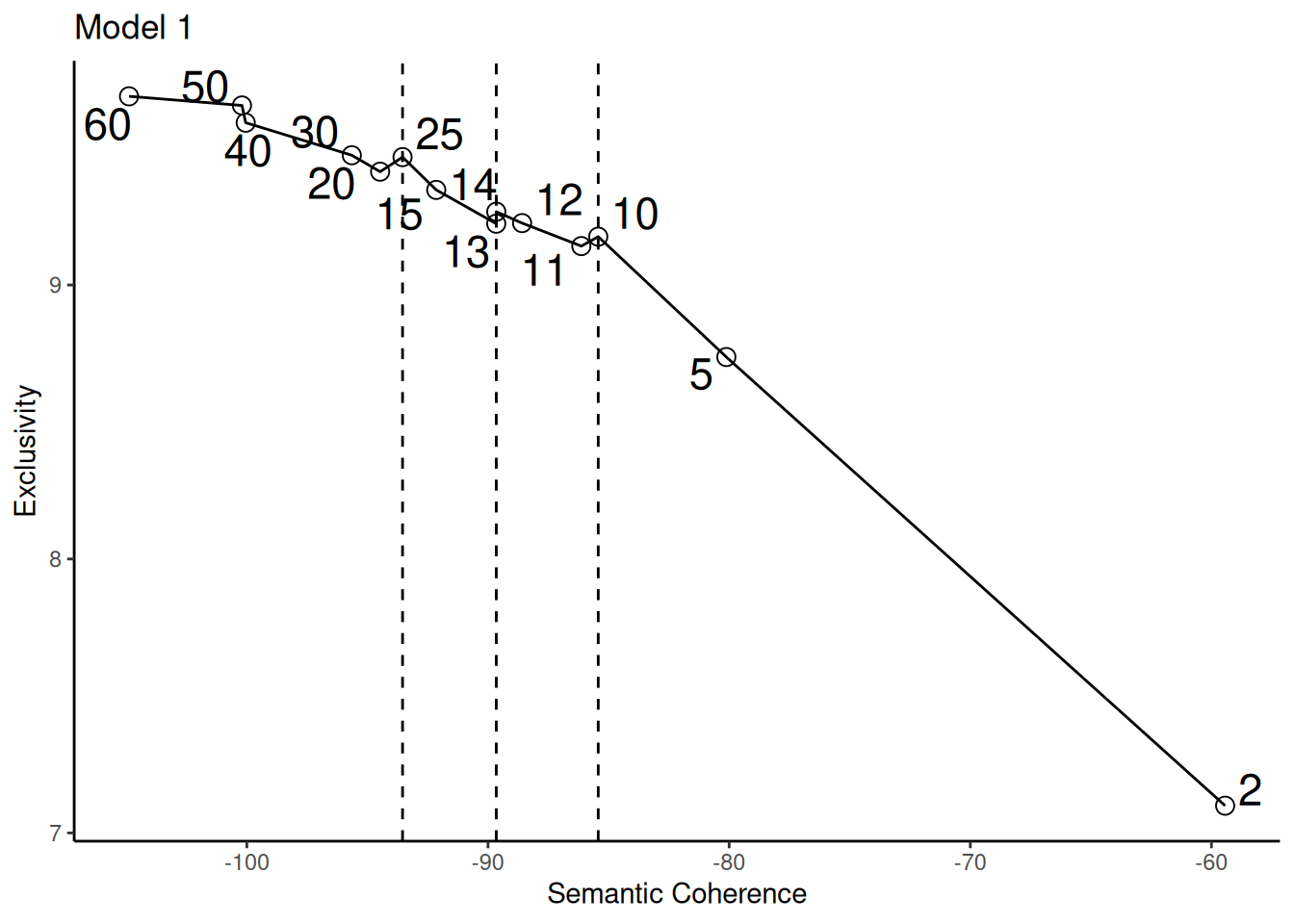
Kuhn (2018) also chose the amount of topics using the same type of graph.
15 topics
# ------------------------------
## Modeling

stm(documents = pesq_doc$documents,
    vocab = pesq_doc$vocab,
    K = 15,
    data = pesq_doc$meta,
    verbose = F) ->
    pesq_stm_fit

tidytext::tidy(pesq_stm_fit) |>
    dplyr::arrange(beta) |>
    dplyr::group_by(topic) |>
    dplyr::top_n(10, beta) |>
    dplyr::arrange(-beta) |>
    dplyr::select(topic, term) |>
    dplyr::summarise(terms = list(term)) |>
    dplyr::mutate(terms = purrr::map(terms, paste, collapse = ", ")) |>
    tidyr::unnest() ->
    top_terms
## Warning: `cols` is now required when using `unnest()`.
## ℹ Please use `cols = c(terms)`.n_documents <- dim(pesq_stm_fit$theta)[1]
tidytext::tidy(pesq_stm_fit, matrix = "gamma") |>
dplyr::group_by(document) |>
dplyr::arrange(dplyr::desc(gamma)) |>
dplyr::slice_head(n = 1) |>
dplyr::ungroup() |>
dplyr::group_by(topic) |>
dplyr::summarise(topic_proportion = n() / n_documents) ->
topic_proportion
topic_proportion |>
left_join(top_terms, by = "topic") |>
mutate(topic = paste0("Topic ", topic)) |>
dplyr::arrange(dplyr::desc(topic_proportion)) ->
topic_proportion2
topic_proportion2 |>
dplyr::mutate(topic = tolower(.data$topic)) |>
dplyr::mutate(topic = gsub(' ', '_', .data$topic)) |>
dplyr::mutate(topic_proportion = round(.data$topic_proportion, digits = 3)) ->
topic_proportion3
rio::export(topic_proportion3, '~/Sync/pirarucu/topic_proportion.xlsx')
topic_proportion3 |>
DT::datatable(
extensions = 'Buttons',
rownames = F,
options = list(
dom = 'Bfrtip',
pageLength = 15,
buttons = list(list(
extend = 'collection',
buttons = list(list(extend = 'csv', filename = 'data'),
list(extend = 'excel', filename = 'data')),
text = 'Download'))))tidytext::tidy(pesq_stm_fit, matrix = "theta", document_names = pesq_prep$meta$nome_do_projeto) |>
dplyr::left_join(pesq |> dplyr::rename(document = nome_do_projeto)) |>
dplyr::distinct(.keep_all = TRUE) |>
dplyr::arrange(document, topic) ->
gamma_documents
gamma_documents |>
dplyr::group_by(topic) |>
dplyr::arrange(dplyr::desc(gamma)) |>
dplyr::slice_head(n = 200) |>
dplyr::ungroup() ->
gamma_documents
gamma_documents |>
dplyr::mutate(topic = paste('topic', topic, sep = '_')) |>
dplyr::mutate(gamma = round(.data$gamma, digits = 3)) |>
dplyr::select(document, topic, gamma, ano_inicio, descricao_do_projeto) ->
tab_top_15
rio::export(tab_top_15, 'rawfiles/stm_tab_top_15.xlsx')
tab_top_15 |>
DT::datatable(
rownames = FALSE,
filter = 'bottom',
extensions = 'Buttons',
options = list(
dom = 'Blfrtip', pageLength = 5,
columnDefs = list(list(visible = FALSE, targets = c(4))),
buttons = list(list(extend = 'colvis', columns = c(0, 1, 2, 4)))
))References
KUHN, K. D. Using structural topic modeling to identify latent topics and trends in aviation incident reports. Transportation Research Part C: Emerging Technologies, v. 87, p. 105–122, fev. 2018.