
Overview
birddog helps you detect emergence and trace
trajectories in scientific literature and patents. It reads datasets
from OpenAlex and Web of Science (WoS), builds citation-based networks,
identifies groups, and summarizes their dynamics.
The stable release is on CRAN. The development version is available on GitHub: https://github.com/roneyfraga/birddog.

Installation
# stable version (CRAN)
install.packages("birddog")

# development version (GitHub)
# install.packages("remotes")
remotes::install_github("roneyfraga/birddog")Data sources
birddog supports two main data sources:
- OpenAlex: browser search with CSV export, or API via openalexR.
-
Web of
Science: multiple export formats (
.bib,.ris, plain-text.txt, tab-delimited.txt).
OpenAlex via API or CSV
library(openalexR)

# Fetch works from OpenAlex API
url_api <- "https://api.openalex.org/works?page=1&filter=primary_location.source.id:s121026525"

openalexR::oa_request(query_url = url_api) |>
  openalexR::oa2df(entity = "works") |>
  birddog::read_openalex(format = "api") ->
  M

# Or from a CSV export
M <- birddog::read_openalex("path/to/openalex-export.csv", format = "csv")
Web of Science (WoS)
# BibTeX
M <- birddog::read_wos("path/to/savedrecs.bib", format = "bib")

# RIS
M <- birddog::read_wos("path/to/savedrecs.ris", format = "ris")

# Plain text
M <- birddog::read_wos("path/to/savedrecs.txt", format = "txt-plain-text")

# Tab-delimited
M <- birddog::read_wos("path/to/savedrecs.txt", format = "txt-tab-delimited")
Example dataset
We use a biogas dataset from OpenAlex with 57,734 documents as a running example.
# Download from OpenAlex (~15 min)
query_oa <- "( biogas )"

openalexR::oa_fetch(
  entity = "works",
  title_and_abstract.search = query_oa,
  verbose = TRUE
) ->
  papers

M <- birddog::read_openalex(papers, format = "api")
# Pre-computed dataset
url_m <- "https://roneyfraga.com/volume/keep_it/biogas-data/M.rds"
M <- readRDS(url(url_m))
dplyr::glimpse(M)
#> Rows: 57,734
#> Columns: 55
#> $ id                          <chr> "https://openalex.org/W2072823483", "https…
#> $ id_short                    <chr> "W2072823483", "W2109587007", "W2032792259…
#> $ SR                          <chr> "W2072823483", "W2109587007", "W2032792259…
#> $ PY                          <int> 2009, 2008, 2009, 2011, 2018, 2015, 2006, …
#> $ TC                          <int> 2672, 2542, 1616, 1228, 1111, 1540, 667, 9…
#> $ TI                          <chr> "Biogas production: current state and pers…
#> $ DI                          <chr> "https://doi.org/10.1007/s00253-009-2246-7…
#> $ AB                          <chr> NA, "Lignocelluloses are often a major or …
#> $ CR                          <chr> "W1417235137;W1503353321;W1506760845;W1529…
#> $ DE                          <chr> "biogas;digestate;renewable natural gas", …
#> $ AU                          <chr> "PETER WEILAND", "MOHAMMAD J. TAHERZADEH;K…
#> $ DB                          <chr> "openalex_api", "openalex_api", "openalex_…
#> $ title                       <chr> "Biogas production: current state and pers…
#> $ display_name                <chr> "Biogas production: current state and pers…
#> $ authorships                 <list> [<tbl_df[1 x 7]>], [<tbl_df[2 x 7]>], [<t…
#> $ abstract                    <chr> NA, "Lignocelluloses are often a major or …
#> $ doi                         <chr> "https://doi.org/10.1007/s00253-009-2246-7…
#> $ publication_date            <date> 2009-09-23, 2008-09-01, 2009-02-14, 2011-…
#> $ publication_year            <int> 2009, 2008, 2009, 2011, 2018, 2015, 2006, …
#> $ relevance_score             <dbl> 1861.7662, 1781.5554, 1455.7186, 1270.2125…
#> $ fwci                        <dbl> 12.110, 6.397, 17.615, 22.271, 68.880, 115…
#> $ cited_by_count              <int> 2672, 2542, 1616, 1228, 1111, 1540, 667, 9…
#> $ counts_by_year              <list> [<data.frame[14 x 2]>], [<data.frame[14 x…
#> $ cited_by_api_url            <chr> "https://api.openalex.org/works?filter=cit…
#> $ ids                         <list> <"https://openalex.org/W2072823483", "htt…
#> $ type                        <chr> "review", "review", "review", "article", "…
#> $ is_oa                       <lgl> FALSE, TRUE, FALSE, FALSE, TRUE, FALSE, FA…
#> $ is_oa_anywhere              <lgl> FALSE, TRUE, FALSE, FALSE, TRUE, FALSE, FA…
#> $ oa_status                   <chr> "closed", "gold", "closed", "closed", "hyb…
#> $ oa_url                      <chr> NA, "https://www.mdpi.com/1422-0067/9/9/16…
#> $ any_repository_has_fulltext <lgl> FALSE, TRUE, FALSE, FALSE, FALSE, FALSE, F…
#> $ source_display_name         <chr> "Applied Microbiology and Biotechnology", …
#> $ source_id                   <chr> "https://openalex.org/S70979998", "https:/…
#> $ issn_l                      <chr> "0175-7598", "1422-0067", "0960-8524", "09…
#> $ host_organization           <chr> "https://openalex.org/P4310319900", "https…
#> $ host_organization_name      <chr> "Springer Science+Business Media", "Multid…
#> $ landing_page_url            <chr> "https://doi.org/10.1007/s00253-009-2246-7…
#> $ pdf_url                     <chr> NA, "https://www.mdpi.com/1422-0067/9/9/16…
#> $ license                     <chr> NA, NA, NA, NA, "cc-by", NA, NA, NA, NA, N…
#> $ version                     <chr> NA, "publishedVersion", NA, NA, "published…
#> $ referenced_works            <list> <"https://openalex.org/W1417235137", "htt…
#> $ referenced_works_count      <int> 55, 193, 9, 10, 14, 145, 16, 0, 211, 50, 1…
#> $ related_works               <list> <"https://openalex.org/W4387315092", "htt…
#> $ concepts                    <list> [<data.frame[21 x 5]>], [<data.frame[18 x…
#> $ topics                      <list> [<tbl_df[12 x 5]>], [<tbl_df[12 x 5]>], […
#> $ keywords                    <list> [<data.frame[3 x 3]>], [<data.frame[5 x 3…
#> $ is_paratext                 <lgl> FALSE, FALSE, FALSE, FALSE, FALSE, FALSE, …
#> $ is_retracted                <lgl> FALSE, FALSE, FALSE, FALSE, FALSE, FALSE, …
#> $ language                    <chr> "en", "en", "en", "en", "en", "en", "en", …
#> $ grants                      <list> NA, NA, NA, NA, NA, NA, NA, NA, NA, NA, <…
#> $ apc                         <list> [<data.frame[2 x 5]>], [<data.frame[2 x 5…
#> $ first_page                  <chr> "849", "1621", "5478", "1633", "457", "540…
#> $ last_page                   <chr> "860", "1651", "5484", "1645", "472", "555…
#> $ volume                      <chr> "85", "9", "100", "35", "129", "45", "32",…
#> $ issue                       <chr> "4", "9", "22", "5", NA, NA, "8", "05", NA…
Citation network
Build a citation network to map the relationships between documents. Direct citation captures time-ordered influence; bibliographic coupling groups papers that share references.
net <- birddog::sniff_network(M, type = "direct citation")
net |>
  tidygraph::activate(nodes) |>
  dplyr::select(name, AU, PY, TI, TC) |>
  dplyr::arrange(dplyr::desc(TC))
#> # A tbl_graph: 29490 nodes and 197059 edges
#> #
#> # A directed simple graph with 297 components
#> #
#> # Node Data: 29,490 × 5 (active)
#>    name        AU                                                 PY TI       TC
#>    <chr>       <chr>                                           <int> <chr> <int>
#>  1 W2072823483 PETER WEILAND                                    2009 Biog…  2672
#>  2 W2109587007 MOHAMMAD J. TAHERZADEH;KEIKHOSRO KARIMI          2008 Pret…  2542
#>  3 W2125363721 DAVID SCHMEIDLER                                 1969 The …  1873
#>  4 W2089274821 İRINI ANGELIDAKI;M. M. ALVES;DAVID BOLZONELLA;…  2009 Defi…  1857
#>  5 W2075740579 PERRY L. MCCARTY;JAEHO BAE;JEONGHWAN KIM         2011 Dome…  1670
#>  6 W2032792259 JENS BO HOLM‐NIELSEN;TEODORITA AL SEADI;PIOTR …  2009 The …  1616
#>  7 W2024397118 CHUNLAN MAO;YONGZHONG FENG;XIAOJIAO WANG;GUANG…  2015 Revi…  1540
#>  8 W2043402970 YI ZHENG;JIA ZHAO;FUQING XU;YEBO LI              2014 Pret…  1238
#>  9 W2018893323 ELINE RYCKEBOSCH;MARGRIET DROUILLON;HAN VERVAE…  2011 Tech…  1228
#> 10 W2111419835 CUNSHENG ZHANG;HAIJIA SU;JAN BAEYENS;TIANWEI T…  2014 Revi…  1173
#> # ℹ 29,480 more rows
#> #
#> # Edge Data: 197,059 × 2
#>    from    to
#>   <int> <int>
#> 1     1    48
#> 2     1    80
#> 3     1    77
#> # ℹ 197,056 more rows
Components
Identify connected components to eliminate disconnected documents that do not share the same bibliographic references.
comps <- birddog::sniff_components(net)
comps$components |>
  dplyr::slice_head(n = 5) |>
gt::gt()| component | quantity_publications | average_age |
|---|---|---|
| c1 | 28820 | 2016.840 |
| c2 | 27 | 2018.444 |
| c3 | 7 | 2014.857 |
| c4 | 7 | 2011.857 |
| c5 | 7 | 2019.286 |
Groups (community detection)
Detect research communities within the citation network. Each group represents a cluster of related publications.
groups <- birddog::sniff_groups(
  comps,
  algorithm = "fast_greedy",
  min_group_size = 30,
  seed = 888L
)
groups$aggregate |>
gt::gt()| group | quantity_papers | average_age |
|---|---|---|
| c1g1 | 6448 | 2017.027 |
| c1g2 | 4157 | 2015.351 |
| c1g3 | 2960 | 2016.728 |
| c1g4 | 2893 | 2017.972 |
| c1g5 | 1937 | 2017.712 |
| c1g6 | 1805 | 2015.425 |
| c1g7 | 1588 | 2017.868 |
| c1g8 | 1529 | 2017.650 |
| c1g9 | 1289 | 2016.700 |
| c1g10 | 924 | 2017.745 |
| c1g11 | 853 | 2017.613 |
| c1g12 | 818 | 2017.555 |
| c1g13 | 598 | 2015.572 |
| c1g14 | 442 | 2017.713 |
| c1g15 | 295 | 2011.854 |
| c1g16 | 47 | 2013.319 |
| c1g17 | 31 | 2019.548 |
Group attributes
Summarize group-level statistics including publication trends and growth rates.
# ~2 min
groups_attributes <- birddog::sniff_groups_attributes(
  groups,
  growth_rate_period = 2010:2024,
  show_results = FALSE
)
groups_attributes$attributes_table| Groups Attributes | |||||
| Group | Publications | Average age1 | Growth rate2 | Doubling time3 | Horizon plot4 |
|---|---|---|---|---|---|
| c1g1 | 6448 | 2017+0m | 6.5 | 11y+1m |  |
| c1g2 | 4157 | 2015+4m | 4.9 | 15y+7m |  |
| c1g3 | 2960 | 2016+9m | 3.7 | 19y+2m |  |
| c1g4 | 2893 | 2017+12m | 9.0 | 8y |  |
| c1g5 | 1937 | 2017+9m | 10.0 | 7y+4m |  |
| c1g6 | 1805 | 2015+5m | 2.9 | 24y+6m |  |
| c1g7 | 1588 | 2017+10m | 8.6 | 8y+5m |  |
| c1g8 | 1529 | 2017+8m | 11.2 | 7y+7m |  |
| c1g9 | 1289 | 2016+8m | 6.0 | 12y+11m |  |
| c1g10 | 924 | 2017+9m | 7.1 | 10y+1m |  |
| c1g11 | 853 | 2017+7m | 6.9 | 10y+5m |  |
| c1g12 | 818 | 2017+7m | 8.4 | 9y+7m |  |
| c1g13 | 598 | 2015+7m | 4.6 | 15y+4m |  |
| c1g14 | 442 | 2017+9m | 11.3 | 6y+6m |  |
| c1g15 | 295 | 2011+10m | 4.8 | 15y+8m |  |
| c1g16 | 47 | 2013+4m | 1.3 | 54y+6m |  |
| c1g17 | 31 | 2019+7m | 16.3 | 5y+7m |  |
| 1 Average publication year: For example, '2016+7m' means that the articles were published, on average, in 2016 plus seven months. | |||||
| 2 Growth rate percentage year. Calculated by exp(b1)-1 where b1 is the econometric model coefficient. Time span, 2010 until 2024. | |||||
| 3 y = years, m = months. Calculated by ln(2)/b1 where b1 is the econometric model coefficient. | |||||
| 4 Publications between 2010 and 2024. Chart type horizon plot. | |||||
| Source: OpenAlex. Data extracted, organized and estimated by the authors. | |||||
Group keywords
Explore the most frequent keywords in each group.
groups_keywords <- birddog::sniff_groups_keywords(groups)

groups_keywords |>
  dplyr::filter(group %in% c('c1g1', 'c1g2', 'c1g3')) |>
gt::gt()| group | term_freq | term_tfidf |
|---|---|---|
| c1g1 | biogas (5702); biogas production (2089); digestion (942); mesophile (785); food waste (644); biodegradable waste (563); cow dung (515); sewage sludge (498); hydraulic retention time (336); digestate (308); lignocellulosic biomass (261); total dissolved solids (228); hemicellulose (203); (188); hyacinth (168) | food waste [0.004] (644); gompertz function [0.004] (150); hyacinth [0.0036] (168); lignocellulosic biomass [0.0035] (261); steam explosion [0.003] (69); total dissolved solids [0.003] (228); digestion [0.0028] (942); hemicellulose [0.0027] (203); mesophile [0.0024] (785); enzymatic hydrolysis [0.0023] (88); sodium hydroxide [0.0023] (60); corn stover [0.0022] (82); stalk [0.0022] (49); sonication [0.0021] (55); eichhornia crassipes [0.002] (76) |
| c1g2 | biogas (3485); biogas production (847); cow dung (261); (212); biodegradable waste (193); energy source (156); animal waste (146); renewable resource (134); mesophile (120); firewood (109); digestion (102); digestate (99); stove (95); food waste (93); investment (85) | firewood [0.0069] (109); stove [0.0051] (95); diesel generator [0.0048] (46); emergy [0.0048] (33); rural electrification [0.0046] (44); dome (geology) [0.0045] (31); microgrid [0.0044] (50); kerosene [0.0036] (41); liquefied petroleum gas [0.0036] (56); hybrid power [0.0035] (34); energy poverty [0.003] (14); payback period [0.0029] (82); deforestation [0.0028] (27); promotion (chess) [0.0025] (24); consumption [0.0024] (46) |
| c1g3 | biogas (2368); biogas production (588); energy crop (281); silage (221); (217); digestate (213); food waste (97); biodegradable waste (87); cogeneration (84); renewable resource (75); digestion (68); manure management (66); investment (65); hectare (58); sewage sludge (58) | hectare [0.0072] (58); energy crop [0.0049] (281); sweet sorghum [0.0044] (22); arable land [0.0043] (41); silage [0.0039] (221); phalaris arundinacea [0.0033] (11); agricultural land [0.0031] (13); arundo donax [0.0027] (11); manure management [0.0025] (66); crop rotation [0.0024] (12); externality [0.0024] (10); supply chain optimization [0.0024] (10); fodder [0.0024] (19); triticale [0.0023] (22); cogeneration [0.0023] (84) |
Group NLP terms
Extract key phrases from abstracts using natural language processing.
# ~30 min
groups_terms <- birddog::sniff_groups_terms(groups, algorithm = "phrase")
groups_terms$terms_table |>
  dplyr::slice_head(n = 3) |>
gt::gt()| group | term_freq | term_tfidf |
|---|---|---|
| c1g1 | biogas production (6713); anaerobic digestion (5247); methane production (1419); food waste (1344); anaerobic co-digestion (1005); methane yield (922); biogas yield (879); cow dung (818); solid waste (804); sewage sludge (759); volatile solids (668); renewable energy (638); water hyacinth (633); retention time (624); digestion process (567) | water hyacinth [0.0017] (633); anaerobic digestion [0.0016] (5247); thermal pretreatment [0.0013] (123); wheat straw [0.0010] (382); anaerobic co-digestion [0.0010] (1005); hydrodynamic cavitation [0.0009] (66); gompertz model [0.0009] (174); coffee pulp [0.0009] (82); production from rice [0.0008] (59); naoh pretreatment [0.0008] (58); sugarcane bagasse [0.0008] (132); mixing ratios [0.0008] (107); rumen fluid [0.0008] (147); orange peel [0.0007] (53); crude glycerol [0.0007] (84) |
| c1g2 | biogas production (1747); renewable energy (1348); anaerobic digestion (988); biogas plants (726); biogas plant (654); biogas technology (638); cow dung (572); energy sources (512); rural areas (388); organic waste (360); case study (343); biogas digester (331); solid waste (328); waste management (318); energy source (290) | technology adoption [0.0022] (83); rural households [0.0021] (102); household biogas [0.0020] (241); domestic biogas [0.0018] (91); biogas digesters [0.0018] (253); cassava peels [0.0018] (87); biogas technology adoption [0.0017] (62); household energy [0.0016] (81); biogas technology [0.0016] (638); rural biogas [0.0015] (73); rural household [0.0014] (84); biogas adoption [0.0014] (51); hybrid system [0.0013] (115); adoption of biogas [0.0013] (81); adoption of biogas technology [0.0013] (47) |
| c1g3 | biogas production (1711); anaerobic digestion (1040); biogas plants (1010); renewable energy (656); biogas plant (638); life cycle (420); greenhouse gas (351); agricultural biogas (321); energy production (301); cycle assessment (300); life cycle assessment (274); energy crops (266); energy sources (261); case study (247); dry matter (217) | cross ref [0.0072] (191); lt ;w [0.0053] (140); lt ;w :lsdexception [0.0041] (109); ;w :lsdexception [0.0041] (109); 2021 cross [0.0031] (82); cup plant [0.0030] (78); 2020 cross [0.0025] (67); agricultural biogas plants [0.0021] (151); 2022 cross [0.0021] (55); operations research [0.0021] (55); silage maize [0.0020] (69); 2019 cross [0.0019] (50); 2021 cross ref [0.0018] (47); energy crops [0.0015] (266); agricultural biogas [0.0015] (321) |
Hubs
Classify documents by their role in the network using the Zi-Pi method. Hub documents connect different research communities.
# ~20 min
groups_hubs <- birddog::sniff_groups_hubs(groups)
groups_hubs |>
  dplyr::filter(zone != "noHub") |>
  dplyr::mutate(Zi = round(Zi, 2), Pi = round(Pi, 2)) |>
  dplyr::arrange(dplyr::desc(zone), dplyr::desc(Zi)) |>
  dplyr::slice_head(n = 15) |>
  gt::gt() |>
  gt::text_transform(
    locations = gt::cells_body(columns = name),
    fn = function(x) {
      glue::glue('<a href="https://openalex.org/{x}" target="_blank">{x}</a>')
    }
)| group | name | TC | Ki | ki | Zi | Pi | zone |
|---|---|---|---|---|---|---|---|
| c1g1 | W2024397118 | 1540 | 524 | 243 | 17.45 | 0.75 | R7 |
| c1g6 | W2072823483 | 2672 | 1101 | 217 | 17.20 | 0.87 | R7 |
| c1g3 | W1972749747 | 737 | 344 | 138 | 13.67 | 0.78 | R7 |
| c1g3 | W2794649776 | 1111 | 523 | 127 | 12.54 | 0.86 | R7 |
| c1g1 | W1606100078 | 939 | 410 | 154 | 10.90 | 0.81 | R7 |
| c1g5 | W2032792259 | 1616 | 551 | 97 | 9.03 | 0.88 | R7 |
| c1g13 | W1985829371 | 227 | 89 | 34 | 8.20 | 0.78 | R7 |
| c1g1 | W2730727434 | 527 | 208 | 79 | 5.38 | 0.79 | R7 |
| c1g12 | W2029511769 | 308 | 96 | 34 | 5.04 | 0.78 | R7 |
| c1g13 | W2338842862 | 132 | 50 | 21 | 4.83 | 0.78 | R7 |
| c1g1 | W2049325764 | 385 | 163 | 64 | 4.27 | 0.79 | R7 |
| c1g5 | W2156879463 | 437 | 119 | 45 | 3.96 | 0.78 | R7 |
| c1g3 | W2798048710 | 329 | 160 | 43 | 3.93 | 0.82 | R7 |
| c1g1 | W2276289647 | 292 | 131 | 59 | 3.90 | 0.76 | R7 |
| c1g8 | W1912164921 | 488 | 132 | 34 | 3.82 | 0.85 | R7 |
Group influence
sniff_groups_influence() lifts the internal citations to
the group level and measures how much each group’s output flows into
every other’s. Influence is directional – if group B’s papers cite group
A’s, knowledge flows A to B – so the cross-citation matrix is
asymmetric, the directed twin of the confluence matrix. Each ordered
pair carries four size-corrected indices (debt, audience, Salton,
surprise); the net flow (citations one way minus the reciprocal) and the
balance (received minus made) classify every group as a source, a broker
or a sink.
influence <- birddog::sniff_groups_influence(groups)

influence$groups |>
gt::gt()| group | received | made | balance | role |
|---|---|---|---|---|
| c1g6 | 15071 | 12833 | 2238 | source |
| c1g3 | 21641 | 19449 | 2192 | source |
| c1g4 | 27778 | 27130 | 648 | source |
| c1g1 | 47818 | 47256 | 562 | source |
| c1g5 | 10840 | 10567 | 273 | source |
| c1g16 | 131 | 135 | -4 | sink |
| c1g17 | 73 | 79 | -6 | sink |
| c1g10 | 6645 | 6661 | -16 | sink |
| c1g15 | 1104 | 1128 | -24 | sink |
| c1g13 | 2278 | 2349 | -71 | sink |
| c1g11 | 1621 | 1733 | -112 | sink |
| c1g14 | 3006 | 3631 | -625 | sink |
| c1g9 | 8796 | 9536 | -740 | sink |
| c1g12 | 3803 | 4757 | -954 | sink |
| c1g2 | 26410 | 27426 | -1016 | sink |
| c1g8 | 8601 | 9660 | -1059 | sink |
| c1g7 | 10493 | 11779 | -1286 | sink |
plot_groups_influence_matrix() is the directed
counterpart of plot_trajectory_confluence_matrix(): rows
are the citing group (“is influenced”), columns the cited group (“the
influencer”), and a cell and its mirror across the diagonal are the two
directions of one pair. Because intra-group citation dominates,
self = FALSE drops the diagonal and sharpens the
between-group surprise.
influence_between <- birddog::sniff_groups_influence(groups, self = FALSE)

birddog::plot_groups_influence_matrix(influence_between, fill = "surprise", x_angle = 45)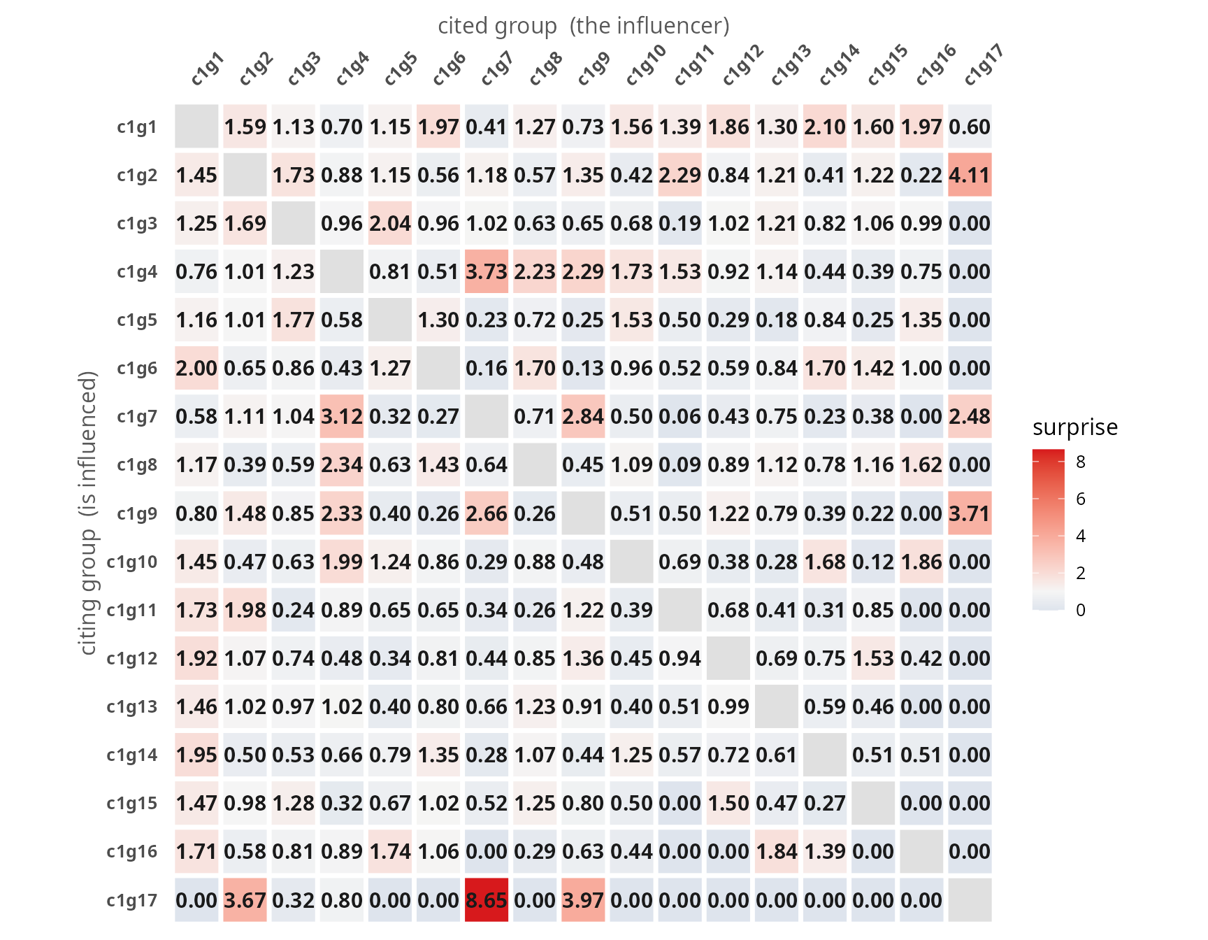
plot_groups_influence_network() renders the same net
flow as a node-link spine rather than a matrix: an arrow from each
source to the group it leads, with nodes coloured by role and edges
weighted by the net flow – the backbone view that complements the
cell-by-cell matrix above.
Indexes
birddog tracks each group’s pace of change and thematic
spread as year-by-year indexes.
Citation Cycle Time
Measure the pace of change in each group by tracking how old the cited references are over time.
# ~1.5 min
groups_cct <- birddog::sniff_cct(
  groups,
  scope = "groups",
  start_year = 2000,
  end_year = 2024
)

groups_cct$plots[["c1g3"]]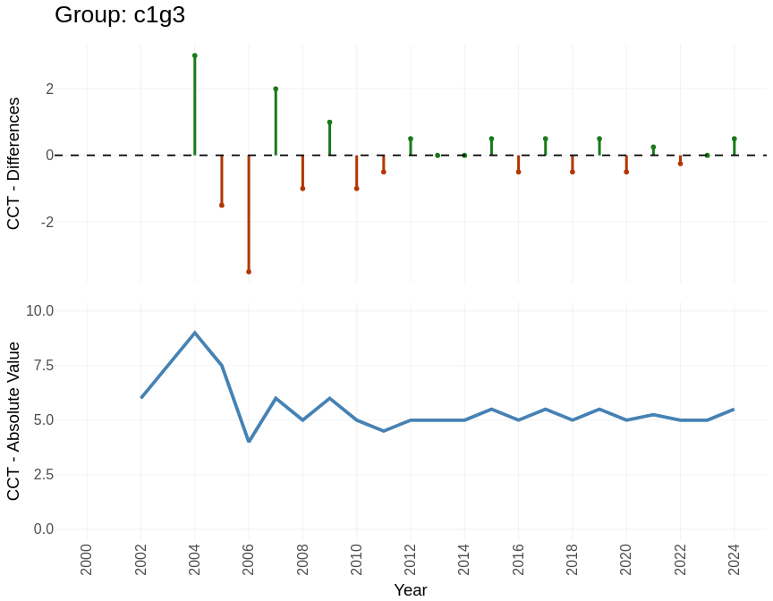
Entropy
Track keyword diversity within each group over time. Increasing entropy signals thematic diversification; decreasing entropy signals convergence.
groups_entropy <- birddog::sniff_entropy(
  groups,
  scope = "groups",
  start_year = 2000,
  end_year = 2024
)

groups_entropy$plots[["c1g3"]]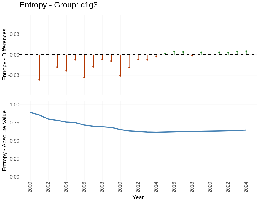
Group lineage
Groups are a stock: each year’s community is recomputed from scratch.
To trace how a community evolves, birddog builds cumulative
networks year by year and tracks each final-year group backwards through
the earlier cuts.
# ~2 min
groups_cumulative <- birddog::sniff_groups_cumulative(groups)
plot_groups_map() lays out the final cumulative network
and colours every document by its group.
birddog::plot_groups_map(groups_cumulative)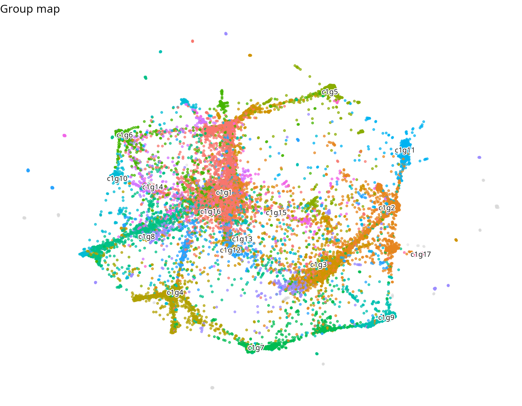
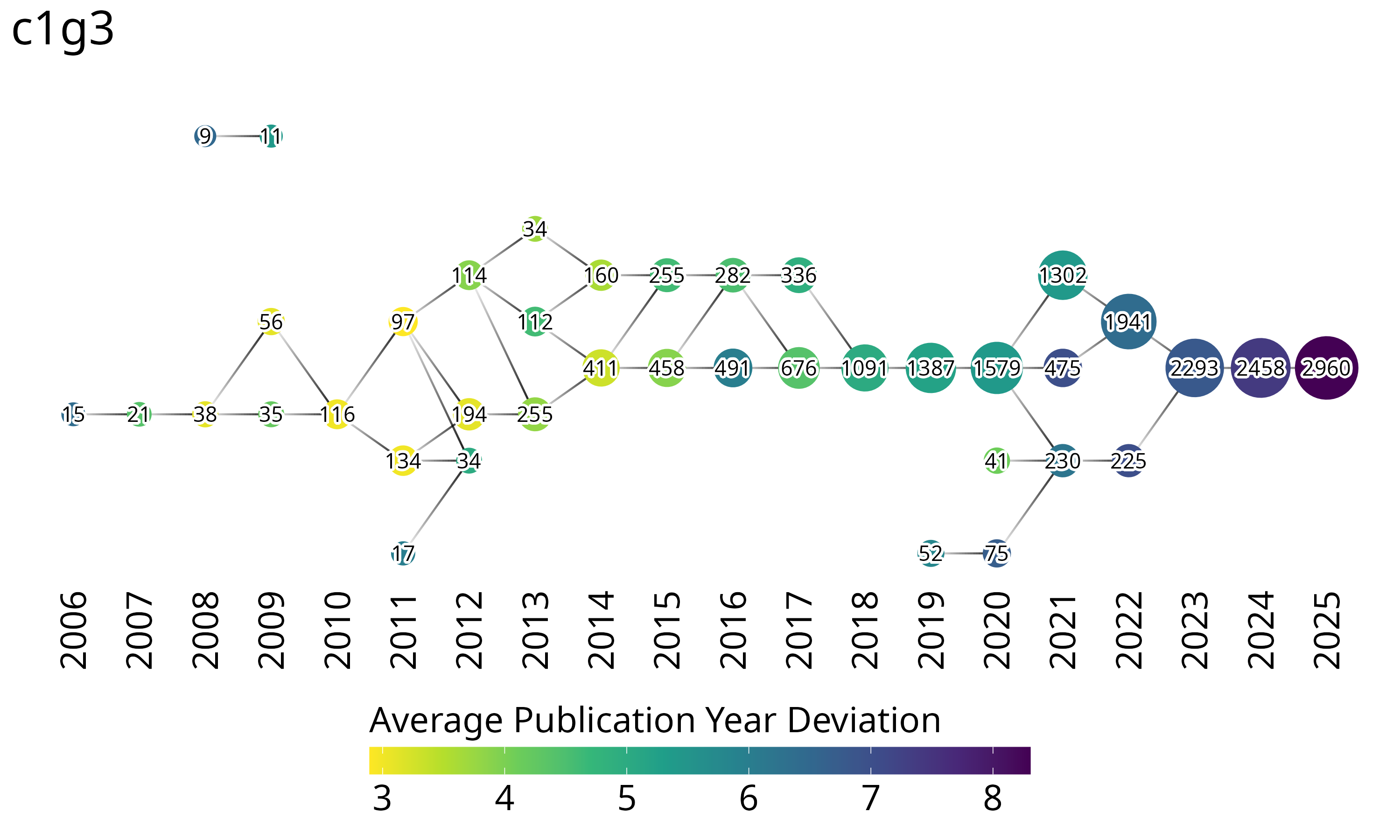
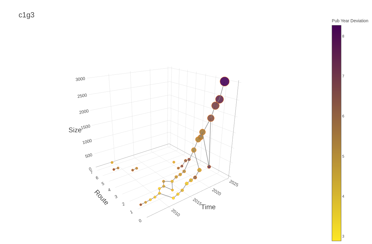
sniff_groups_lineage() tracks each final-year group
backwards through the cumulative cuts;
plot_groups_lineage_2d() and
plot_groups_lineage_3d() draw one group’s lineage at a
time.
suppressMessages({
  groups_lineage <- birddog::sniff_groups_lineage(groups_cumulative)
})

birddog::plot_groups_lineage_2d(
  groups_lineage,
  group = "c1g3",
  label_vertical_position = -2
)

birddog::plot_groups_lineage_3d(
  groups_lineage,
  group = "c1g3"
)
Trajectories
The lineage view follows one group at a time. Trajectories are a
flow: sniff_trajectory_dag() reads the whole
cumulative-clustering history at once and builds the temporal DAG of
cluster-year nodes.
dag <- birddog::sniff_trajectory_dag(groups_lineage)

dag
#> <birddog_dag> 410 group-year nodes, 537 edges, 1993-2025
plot_groups_per_year() counts the groups alive in each
yearly cut; plot_trajectory_dag() draws the full
node-and-edge DAG.
birddog::plot_groups_per_year(dag)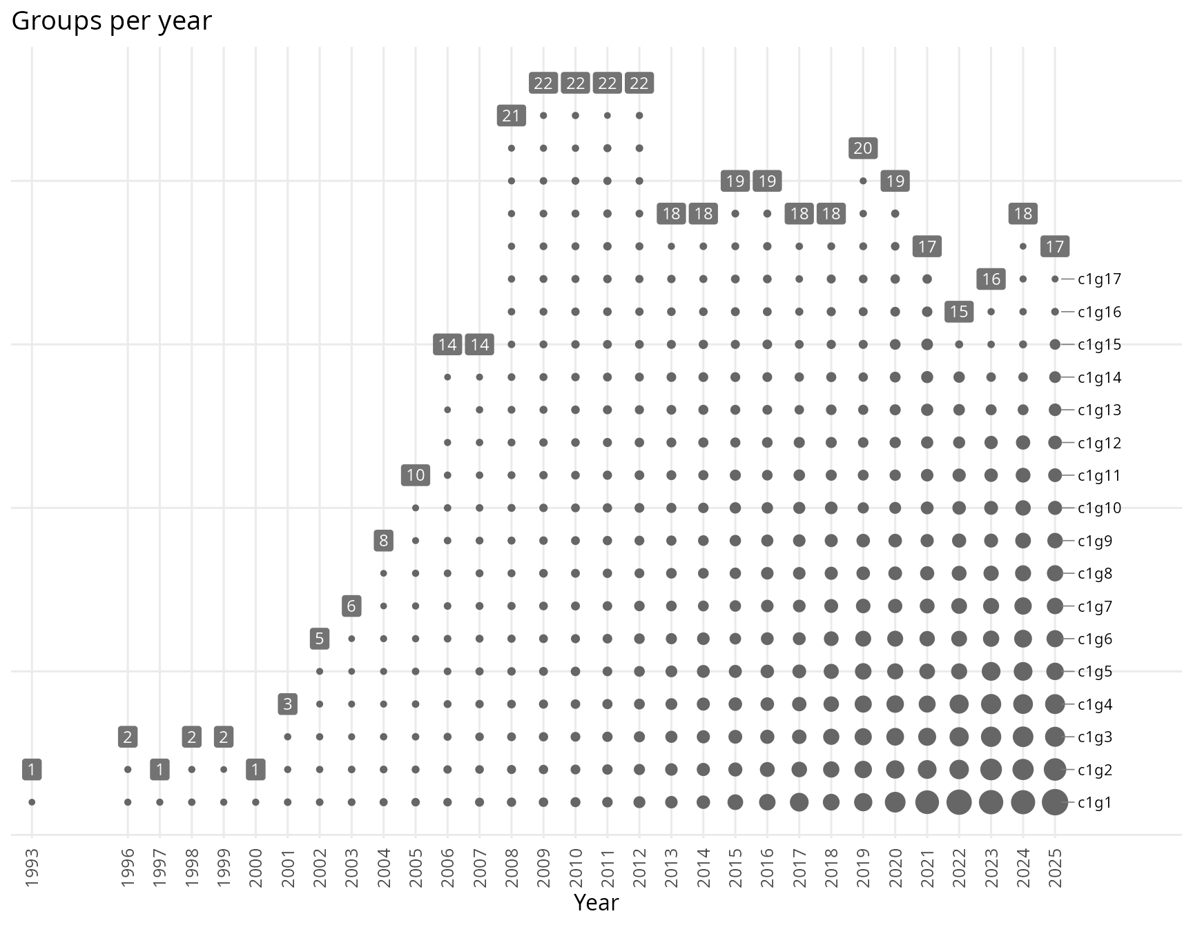
birddog::plot_trajectory_dag(dag)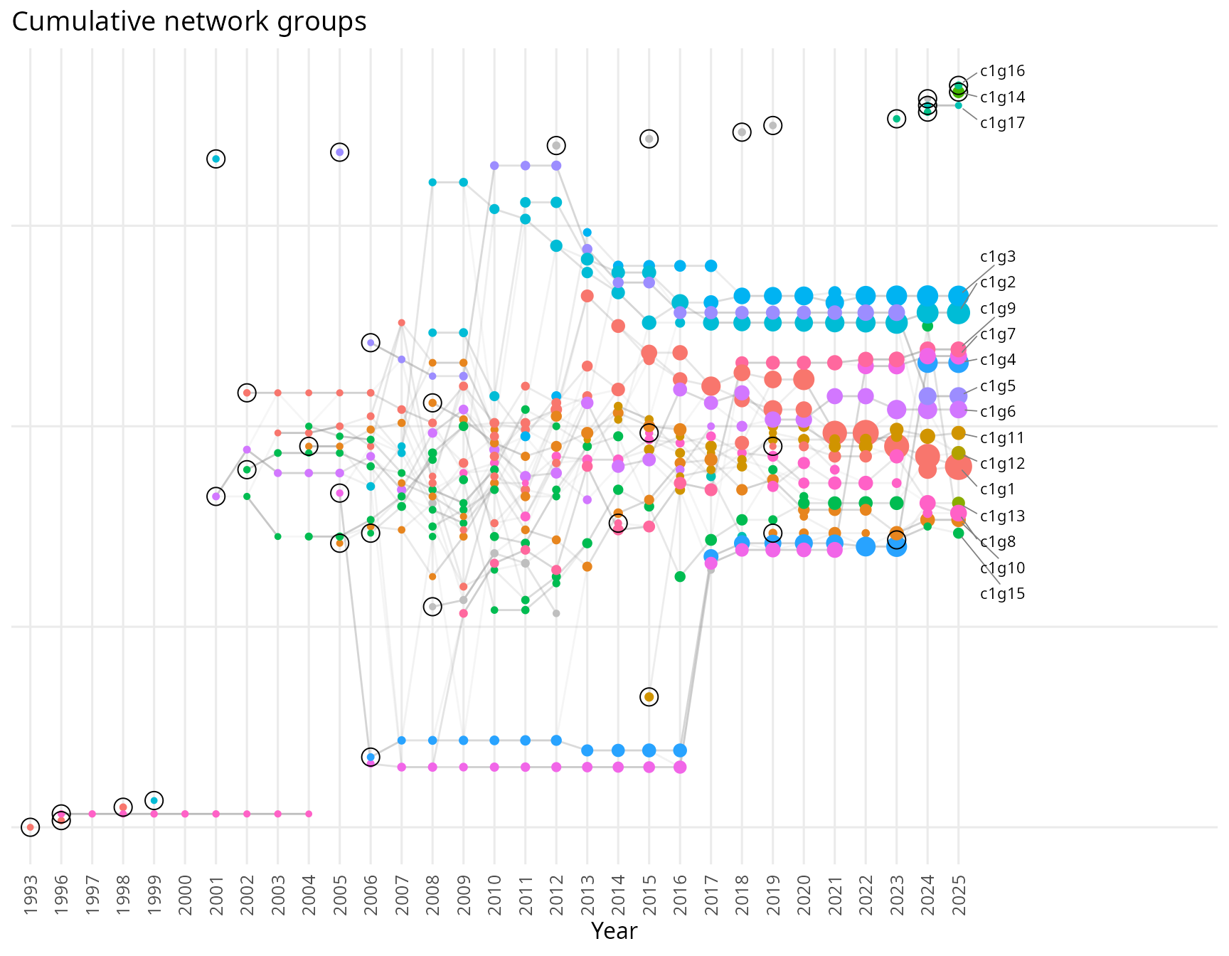
Braid
sniff_trajectory_braid() decomposes that DAG into
trajectories. A trajectory that reaches the final year is
central (one per final group, named
tr::c1g1, tr::c1g2, and so on). Every other
trajectory is intermediate (tr1 …
trN, stored as type == "absorbed"): it merges
into a central one before the end. Groups are stock, trajectories are
flow.
braid <- birddog::sniff_trajectory_braid(dag)

braid
#> <birddog_flow> 17 central + 68 absorbed trajectories, last year 2025
#> # A tibble: 5 × 4
#>   traj_id  start   end  size
#>   <chr>    <int> <int> <int>
#> 1 tr::c1g1  2010  2025  9933
#> 2 tr::c1g2  2007  2025  6327
#> 3 tr::c1g3  2017  2025  4985
#> 4 tr::c1g4  2006  2025  4834
#> 5 tr::c1g6  2001  2025  4467
braid$trajectories has one row per trajectory.
Absorption is transitive, so the intermediate trajectories form a
confluence tree under the centrals.
subset() focuses a flow on a watershed – a central
trajectory and its whole tributary subtree – or on any predicate over
braid$trajectories, and the result is still a valid flow
(the pruning call is recorded and shown when you print it).
# keep the central of group c1g3 and every trajectory that feeds it
watershed <- subset(braid, target = "tr::c1g3")

watershed
#> <birddog_flow> 1 central + 2 absorbed trajectories, last year 2025
#> (pruned: subset.birddog_flow(braid, target = "tr::c1g3"))
#> # A tibble: 1 × 4
#>   traj_id  start   end  size
#>   <chr>    <int> <int> <int>
#> 1 tr::c1g3  2017  2025  4985
Channel
sniff_trajectory_channel() is a sibling detector over
the same DAG. Instead of braiding tributaries into each central, it
routes one global optimal-path backbone per final group, an alternative
decomposition that keeps the same birddog_flow
contract.
channel <- birddog::sniff_trajectory_channel(dag)

channel
#> <birddog_flow> 17 central + 84 absorbed trajectories, last year 2025
#> # A tibble: 5 × 4
#>   traj_id  start   end  size
#>   <chr>    <int> <int> <int>
#> 1 tr::c1g1  2024  2025  6692
#> 2 tr::c1g2  2016  2025  5631
#> 3 tr::c1g3  2021  2025  4381
#> 4 tr::c1g4  2020  2025  4321
#> 5 tr::c1g6  2017  2025  3953
Confluence
sniff_trajectory_confluence() turns the flow into
render-ready data and plot_trajectory_confluence() draws
the whole forest: each central trajectory is a river, each intermediate
trajectory a tributary merging in at its handoff year.
conf <- birddog::sniff_trajectory_confluence(braid)

birddog::plot_trajectory_confluence(conf, target = c('tr::c1g1', 'tr::c1g2', 'tr::c1g3'))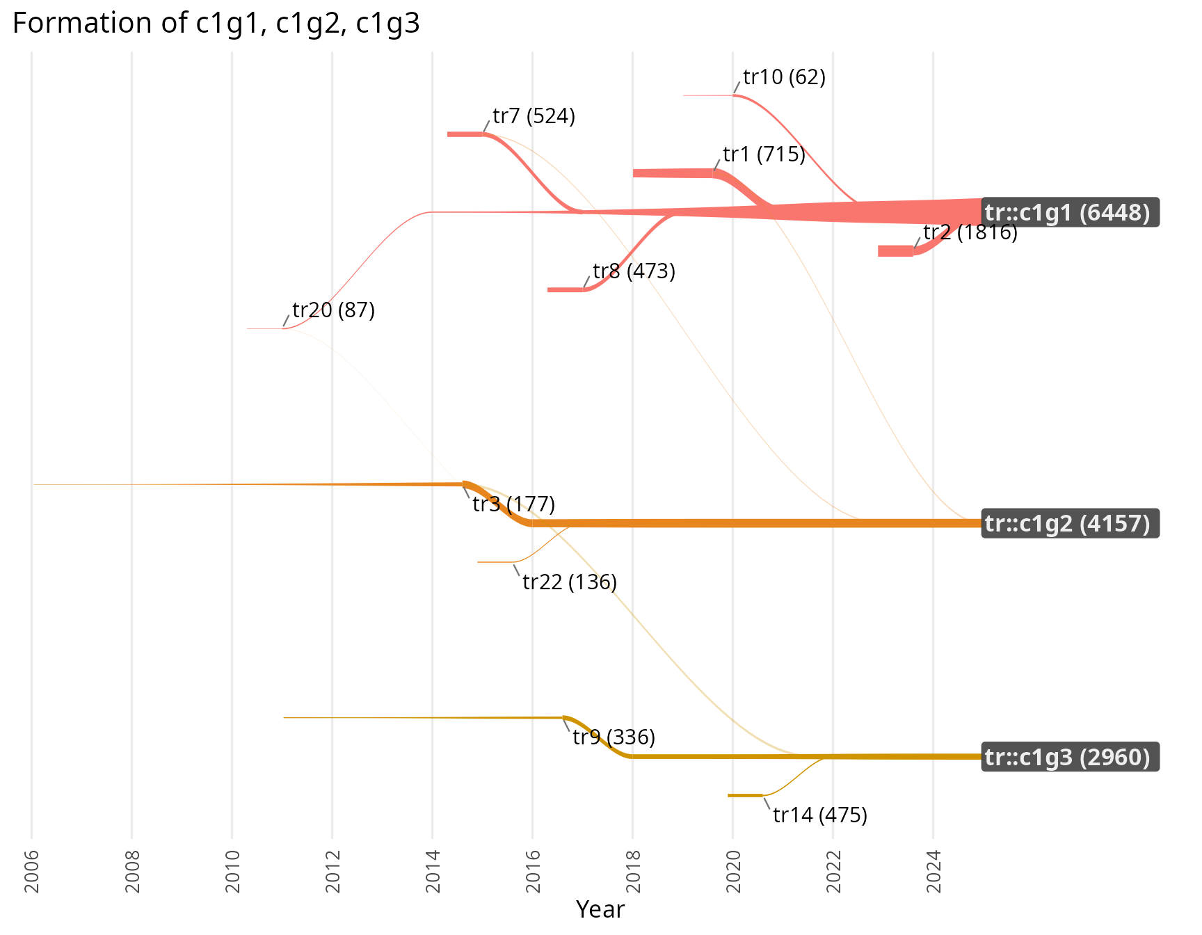
Trajectory lines
plot_trajectory_lines_2d() is the line counterpart of
the confluence delta: every trajectory is a variable-width line on the
year-aware Sugiyama layout, widening with the documents it accumulates.
Targeting a central draws it and the trajectories that feed it; the
legend reports how many papers of each feeder’s terminal cohort reached
the final group. Where
plot_trajectory_confluence(conf, target = ...) keeps only
the direct tributaries (depth = 1), the lines view follows
the whole tributary subtree – feeders and feeders of feeders – so a
targeted central shows more lines here than in the confluence delta.
Open the delta to every depth with
plot_trajectory_confluence(conf, target = "tr::c1g3", depth = Inf).
birddog::plot_trajectory_lines_2d(braid, target = "tr::c1g3")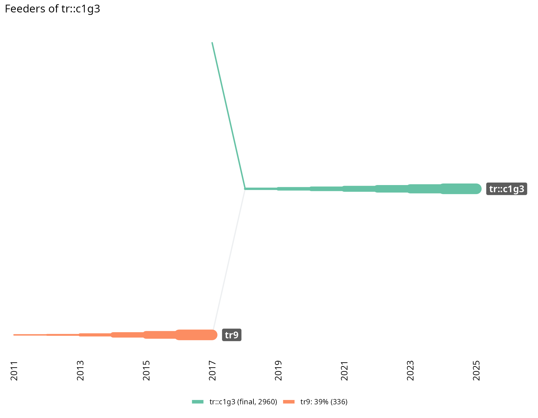
plot_trajectory_lines_3d() is the interactive plotly
version of the same view: x = year, y = route (the Sugiyama branching
coordinate), z = cumulative tracked documents.
birddog::plot_trajectory_lines_3d(braid, target = "tr::c1g3")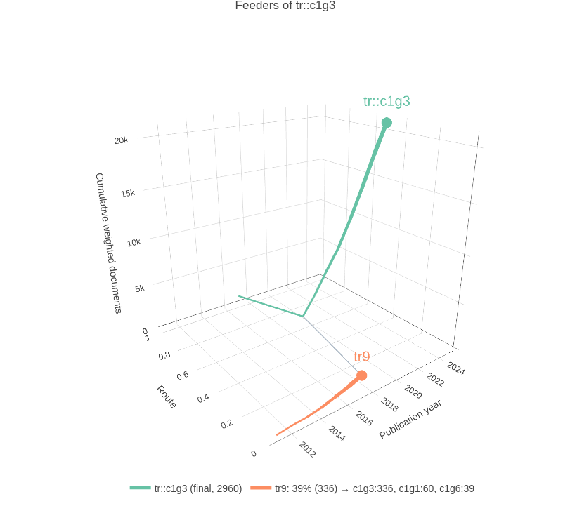
Where an intermediate trajectory’s papers go
A trajectory can stop before the final year, but with cumulative
clustering its papers never leave the network: they are re-grouped each
year. sniff_trajectory_destination() follows a trajectory’s
terminal cohort forward and reports where the papers land, split by
final group. Here tr9 (2011-2017, handed off in 2018) is
mostly captured by group c1g3: 336 of its 502 terminal
papers end in c1g3’s final community, and none drop out of
the network.
# where do the papers of trajectory tr9 go?
dest <- birddog::sniff_trajectory_destination(braid, source = "tr9")

dest$destination
#> # A tibble: 13 × 3
#>    g_final     n    prop
#>    <chr>   <int>   <dbl>
#>  1 c1g3      336 0.669
#>  2 c1g1       60 0.120
#>  3 c1g6       39 0.0777
#>  4 c1g5       16 0.0319
#>  5 c1g13      13 0.0259
#>  6 c1g2       13 0.0259
#>  7 c1g15       6 0.0120
#>  8 c1g4        6 0.0120
#>  9 c1g11       5 0.00996
#> 10 c1g12       2 0.00398
#> 11 c1g14       2 0.00398
#> 12 c1g8        2 0.00398
#> 13 c1g9        2 0.00398

birddog::plot_trajectory_dispersion(dest)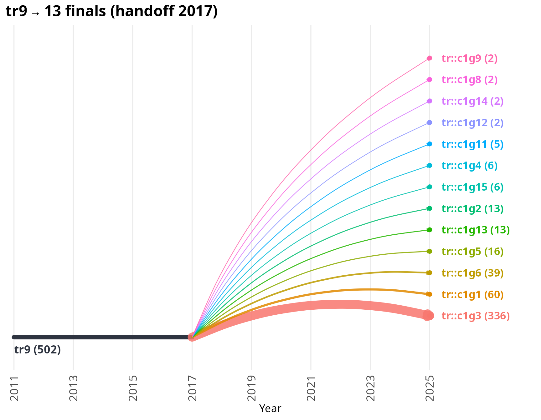
Which trajectories formed a central one
The mirror of the previous analysis: stand at a central trajectory
and ask which trajectories fed into it.
sniff_trajectory_formation() returns the target’s direct
tributaries in the confluence tree.
plot_trajectory_formation() draws the target as a
cumulative river with each feeder merging at its handoff year. Two
feeders formed tr::c1g3: tr9, handed off in
2018, and tr14, handed off in 2022; the labels count each
feeder’s papers that sit in the target’s final community.
# which trajectories formed the central trajectory of group c1g3?
form <- birddog::sniff_trajectory_formation(braid, target = "tr::c1g3")

form$feeders
#> # A tibble: 2 × 12
#>   source_key source_group start_year handoff_year cohort_size     n n_dest
#>   <chr>      <chr>             <int>        <int>       <int> <int>  <int>
#> 1 tr9        c1g3               2011         2018         851   851    336
#> 2 tr14       c1g3               2021         2022         586   246    475
#> # ℹ 5 more variables: size_curve <list>, inflow_curve <list>,
#> #   prop_of_source <dbl>, prop_of_inflow <dbl>, kept <lgl>

birddog::plot_trajectory_formation(form, max_feeders = 8)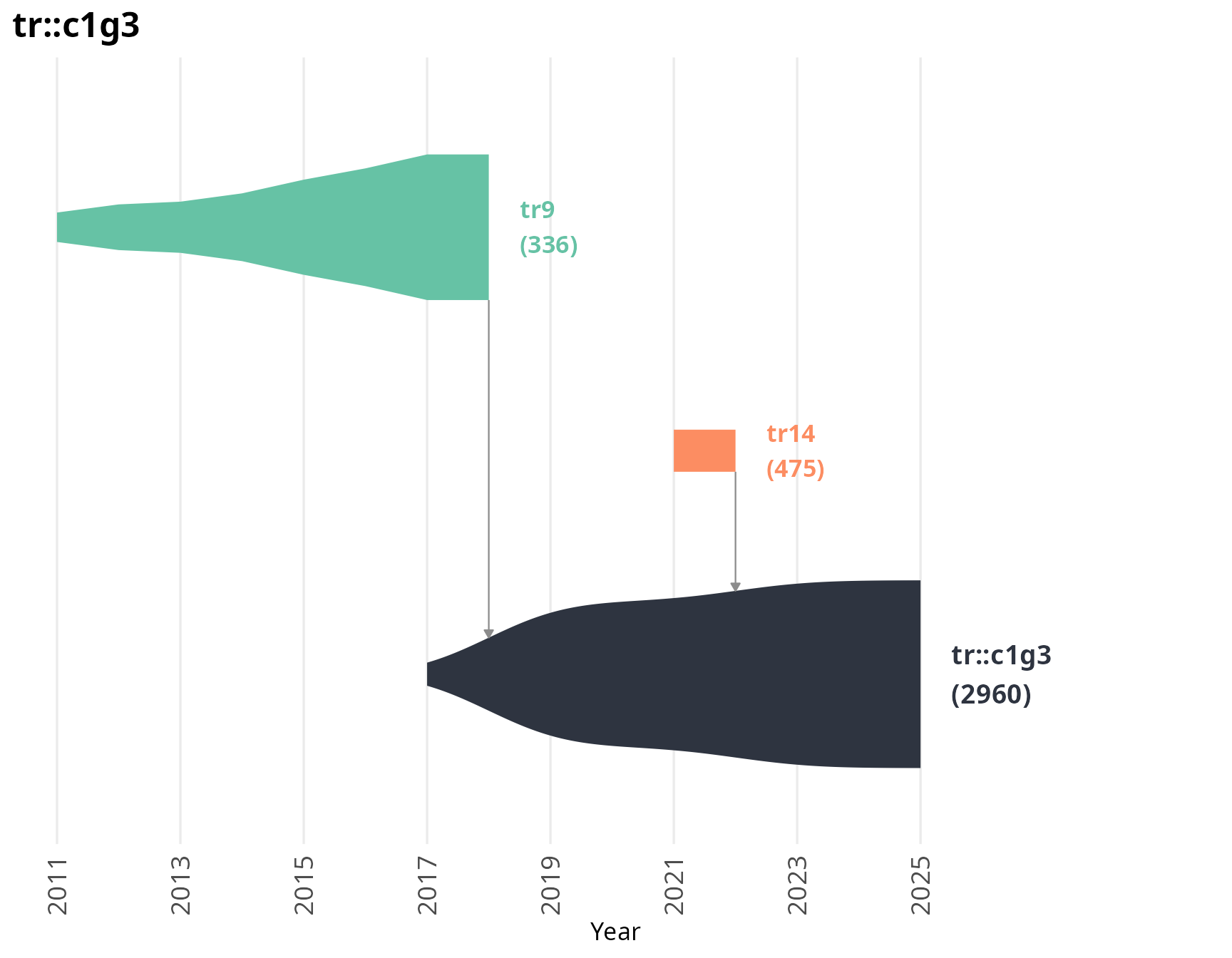
Documents transferred
sniff_trajectory_destination() and
sniff_trajectory_formation() count the papers that crossed;
sniff_trajectory_contribution() lists them. Given an
intermediate trajectory, the year of its terminal cohort, and a central
target, it returns one row per document with in_target
flagging those that reached the target’s final-year community.
# the terminal-cohort year of tr9 (its last node)
yr <- max(as.integer(sub("^y(\\d{4}).*", "\\1",
  braid$trajectories$nodes[[which(braid$trajectories$traj_id == "tr9")]])))

contrib <- birddog::sniff_trajectory_contribution(
  braid,
  source = "tr9",
  year = yr,
  target = "tr::c1g3"
)

contrib |>
  dplyr::summarise(documents = dplyr::n(), in_target = sum(in_target))
#> # A tibble: 1 × 2
#>   documents in_target
#>       <int>     <int>
#> 1       502       336
Self-sufficiency
How much of each central trajectory grew on its own versus being a
confluence of others? sniff_trajectory_self_sufficiency()
reports the share of each central trajectory’s final-year community that
was not delivered by an intermediate tributary: values near 1 mean the
lineage grew endogenously; lower values mean it absorbed many documents
from other communities.
ss <- birddog::sniff_trajectory_self_sufficiency(braid)

ss |>
  dplyr::mutate(self_sufficiency = round(self_sufficiency, 2)) |>
  dplyr::slice_head(n = 10) |>
gt::gt()| central | group | final_size | inflow | self_sufficiency |
|---|---|---|---|---|
| tr::c1g17 | c1g17 | 31 | 0 | 1.00 |
| tr::c1g4 | c1g4 | 2893 | 113 | 0.96 |
| tr::c1g7 | c1g7 | 1588 | 84 | 0.95 |
| tr::c1g9 | c1g9 | 1289 | 72 | 0.94 |
| tr::c1g5 | c1g5 | 1937 | 203 | 0.90 |
| tr::c1g10 | c1g10 | 924 | 102 | 0.89 |
| tr::c1g11 | c1g11 | 853 | 132 | 0.85 |
| tr::c1g6 | c1g6 | 1805 | 333 | 0.82 |
| tr::c1g2 | c1g2 | 4157 | 981 | 0.76 |
| tr::c1g13 | c1g13 | 598 | 178 | 0.70 |
Trajectory dynamics
sniff_trajectory_dynamics() computes growth, novelty,
recruitment and destination indicators per trajectory, then classifies
each one into a dynamic state. Emergence: a central trajectory growing
fast with a high share of recent papers. Convergence: an intermediate
trajectory whose terminal cohort concentrates in a single central one.
Divergence: an intermediate trajectory whose cohort scatters across
several. Dormancy: a central trajectory that stalled, or an intermediate
one whose cohort mostly drops out of the network. Central trajectories
in between are classified as maturity.
dyn <- birddog::sniff_trajectory_dynamics(braid)

birddog::plot_trajectory_dynamics(dyn)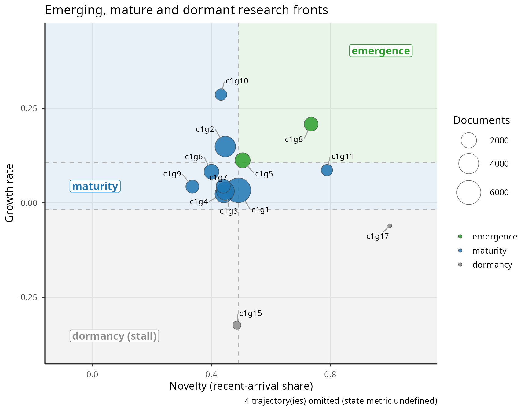
Per-trajectory lenses
sniff_trajectory_dynamics() left-joins optional lenses,
each recomputed from the trajectory’s own documents and supplied as a
per-year list-column: renewal pace
(sniff_trajectory_cct()), keyword diversity
(sniff_trajectory_entropy()) and hub roles
(sniff_trajectory_hubs()). They are built from the corpus
fields keyed by document id.
keywords <- M |>
  dplyr::transmute(document_id = SR, keyword = DE) |>
  tidyr::separate_rows(keyword, sep = ";") |>
  dplyr::mutate(keyword = trimws(keyword)) |>
  dplyr::filter(keyword != "")

references <- M |>
  dplyr::transmute(document_id = SR, PY, CR) |>
  tidyr::separate_rows(CR, sep = ";") |>
  dplyr::mutate(CR = trimws(CR)) |>
  dplyr::filter(CR != "") |>
  dplyr::left_join(
    dplyr::distinct(groups_cct$tracked_cr_py, CR, .keep_all = TRUE), by = "CR") |>
  dplyr::filter(!is.na(CR_PY), PY > CR_PY) |>
  dplyr::transmute(document_id, ref_age = PY - CR_PY)

dyn <- birddog::sniff_trajectory_dynamics(
  braid,
  cct = birddog::sniff_trajectory_cct(braid, references),
  entropy = birddog::sniff_trajectory_entropy(braid, keywords),
  hubs = birddog::sniff_trajectory_hubs(braid, groups_hubs)
)
sniff_trajectory_emergence_owners() then credits each
central trajectory’s emergence to its authors, surfacing the field’s
leaders.
authors <- M |>
  dplyr::transmute(document_id = SR, author = AU) |>
  tidyr::separate_rows(author, sep = ";") |>
  dplyr::mutate(author = trimws(author)) |>
  dplyr::filter(author != "")

birddog::sniff_trajectory_emergence_owners(braid, dyn, authors) |>
  dplyr::mutate(total = round(total, 2), norm = round(norm, 2)) |>
  dplyr::slice_head(n = 10) |>
gt::gt()| author | total | ndocs | norm |
|---|---|---|---|
| İRINI ANGELIDAKI | 401.99 | 261 | 24.88 |
| MARCIN DĘBOWSKI | 301.32 | 154 | 24.28 |
| MARCIN ZIELIŃSKI | 300.96 | 149 | 24.66 |
| RAÚL MUÑOZ | 300.00 | 175 | 22.68 |
| BUDIYONO BUDIYONO | 228.35 | 101 | 22.72 |
| REGINA MAMBELI BARROS | 215.19 | 75 | 24.85 |
| IVAN FELIPE SILVA DOS SANTOS | 202.50 | 69 | 24.38 |
| MOHAMMAD J. TAHERZADEH | 196.98 | 89 | 20.88 |
| KEIKHOSRO KARIMI | 179.71 | 67 | 21.95 |
| VILIS DUBROVSKIS | 176.00 | 100 | 17.60 |
Citation growth per document
Track how individual documents accumulate citations over time to identify fast-growing papers.
# ~11 min
groups_cumulative_citations <- birddog::sniff_groups_cumulative_citations(
  groups,
  min_citations = 2
)
Main Path Analysis
Identify the key route through the citation network, revealing the most influential chain of documents over time.
groups_key_route <- birddog::sniff_key_route(groups, scope = "groups")

groups_key_route[["c1g3"]]$plot

groups_key_route[["c1g3"]]$data |>
  dplyr::select(-name) |>
  gt::gt()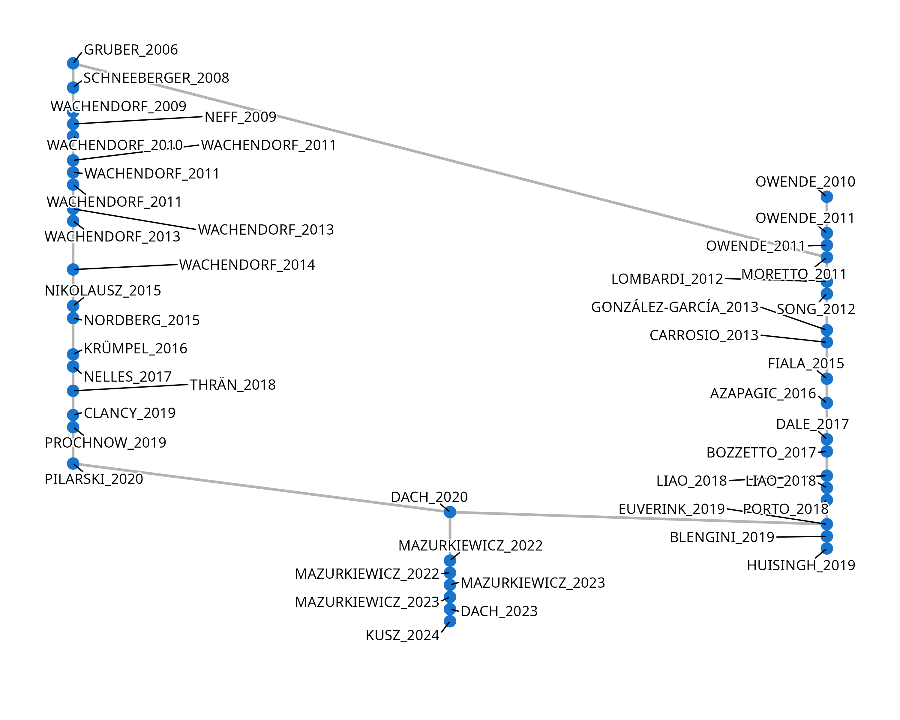
key_route_c1g3_data |>
  dplyr::select(document = name, name2, title = TI) |>
  gt::gt() |>
  gt::text_transform(
    locations = gt::cells_body(columns = document),
    fn = function(x) {
      glue::glue('<a href="https://openalex.org/{x}" target="_blank">{x}</a>')
    }
)| document | name2 | title |
|---|---|---|
| W2008561700 | GRUBER_2006 | Biogas production from maize and dairy cattle manure—Influence of biomass composition on the methane yield |
| W2033886695 | SCHNEEBERGER_2008 | The optimal size for biogas plants |
| W2158862659 | NEFF_2009 | Utilization of semi‐natural grassland through integrated generation of solid fuel and biogas from biomass. I. Effects of hydrothermal conditioning and mechanical dehydration on mass flows of organic and mineral plant compounds, and nutrient balances |
| W2019905517 | WACHENDORF_2009 | Utilization of semi‐natural grassland through integrated generation of solid fuel and biogas from biomass. II. Effects of hydrothermal conditioning and mechanical dehydration on anaerobic digestion of press fluids |
| W1972749747 | OWENDE_2010 | Evaluation of energy efficiency of various biogas production and utilization pathways |
| W2134179273 | WACHENDORF_2010 | Utilization of semi‐natural grassland through integrated generation of solid fuel and biogas from biomass. III. Effects of hydrothermal conditioning and mechanical dehydration on solid fuel properties and on energy and greenhouse gas balances |
| W2003509580 | OWENDE_2011 | Environmental impacts of biogas deployment – Part II: life cycle assessment of multiple production and utilization pathways |
| W1997982003 | OWENDE_2011 | Environmental impacts of biogas deployment – Part I: life cycle inventory for evaluation of production process emissions to air |
| W2023450208 | WACHENDORF_2011 | Integrated generation of solid fuel and biogas from green cut material from landscape conservation and private households |
| W3124542086 | MORETTO_2011 | Investing in biogas: Timing, technological choice and the value of flexibility from input mix |
| W2075790500 | WACHENDORF_2011 | Influence of sward maturity and pre-conditioning temperature on the energy production from grass silage through the integrated generation of solid fuel and biogas from biomass (IFBB): 1. The fate of mineral compounds |
| W2091870505 | WACHENDORF_2011 | Influence of sward maturity and pre-conditioning temperature on the energy production from grass silage through the integrated generation of solid fuel and biogas from biomass (IFBB): 2. Properties of energy carriers and energy yield |
| W2078934777 | SONG_2012 | Life-cycle energy production and emissions mitigation by comprehensive biogas–digestate utilization |
| W2051151463 | LOMBARDI_2012 | Environmental analysis of biogas production systems |
| W2044886835 | WACHENDORF_2013 | Review of concepts for a demand-driven biogas supply for flexible power generation |
| W2064487381 | GONZÁLEZ‐GARCÍA_2013 | Anaerobic digestion of different feedstocks: Impact on energetic and environmental balances of biogas process |
| W2046271618 | CARROSIO_2013 | Energy production from biogas in the Italian countryside: Policies and organizational models |
| W2010747108 | WACHENDORF_2013 | Energetic conversion of European semi-natural grassland silages through the integrated generation of solid fuel and biogas from biomass: Energy yields and the fate of organic compounds |
| W2065522991 | WACHENDORF_2014 | Cost analysis of concepts for a demand oriented biogas supply for flexible power generation |
| W2191399137 | NIKOLAUSZ_2015 | Changing Feeding Regimes To Demonstrate Flexible Biogas Production: Effects on Process Performance, Microbial Community Structure, and Methanogenesis Pathways |
| W2048561114 | NORDBERG_2015 | Demand-Orientated Power Production from Biogas: Modeling and Simulations under Swedish Conditions |
| W1126637212 | FIALA_2015 | CARBON FOOTPRINT OF ELECTRICITY FROM ANAEROBIC DIGESTION PLANTS IN ITALY |
| W2312683967 | AZAPAGIC_2016 | Life Cycle Environmental Impacts of Electricity from Biogas Produced by Anaerobic Digestion |
| W2556832018 | KRÜMPEL_2016 | Demand-driven biogas production in anaerobic filters |
| W2592402297 | NELLES_2017 | Demand-driven biogas production by flexible feeding in full-scale – Process stability and flexibility potentials |
| W2724845225 | BOZZETTO_2017 | Greenhouse gas emissions of electricity and biomethane produced using the Biogasdoneright™ system: four case studies from Italy |
| W2768561067 | DALE_2017 | Sequential crops for food, energy, and economic development in rural areas: the case of Sicily |
| W2805047418 | LIAO_2018 | Anaerobic co-digestion of multiple agricultural residues to enhance biogas production in southern Italy |
| W2794973208 | THRÄN_2018 | Flexible Biogas in Future Energy Systems—Sleeping Beauty for a Cheaper Power Generation |
| W2888708623 | LIAO_2018 | Spatial analysis of feedstock supply and logistics to establish regional biogas power generation: A case study in the region of Sicily |
| W2790521460 | PORTO_2018 | A GIS‐based spatial index of feedstock‐mixture availability for anaerobic co‐digestion of Mediterranean by‐products and agricultural residues |
| W2914822267 | PROCHNOW_2019 | The Future Agricultural Biogas Plant in Germany: A Vision |
| W2988479878 | EUVERINK_2019 | Rambling facets of manure-based biogas production in Europe: A briefing |
| W2969910225 | CLANCY_2019 | Promoting agricultural biogas and biomethane production: Lessons from cross-country studies |
| W2907370432 | HUISINGH_2019 | Investigating energy and environmental issues of agro-biogas derived energy systems: A comprehensive review of Life Cycle Assessments |
| W2941197762 | BLENGINI_2019 | Life Cycle Assessment of a Biogas-Fed Solid Oxide Fuel Cell (SOFC) Integrated in a Wastewater Treatment Plant |
| W3004153001 | PILARSKI_2020 | 15 Years of the Polish agricultural biogas plants: their history, current status, biogas potential and perspectives |
| W3102984777 | DACH_2020 | Biogas Plant Exploitation in a Middle-Sized Dairy Farm in Poland: Energetic and Economic Aspects |
| W4205695009 | MAZURKIEWICZ_2022 | Energy and Economic Balance between Manure Stored and Used as a Substrate for Biogas Production |
| W4309852604 | MAZURKIEWICZ_2022 | Analysis of the Energy and Material Use of Manure as a Fertilizer or Substrate for Biogas Production during the Energy Crisis |
| W4386850198 | MAZURKIEWICZ_2023 | Loss of Energy and Economic Potential of a Biogas Plant Fed with Cow Manure due to Storage Time |
| W4321781369 | DACH_2023 | Reduction of Greenhouse Gas Emissions by Replacing Fertilizers with Digestate |
| W4386913257 | MAZURKIEWICZ_2023 | The Impact of Manure Use for Energy Purposes on the Economic Balance of a Dairy Farm |
| W4405283529 | KUSZ_2024 | The Capacity of Power of Biogas Plants and Their Technical Efficiency: A Case Study of Poland |
Topic modeling (STM)
Detect topics within a group using Structural Topic Modeling, creating sub-groups based on linguistic similarities.
# Prepare STM data (~30 min)
groups_stm_prepare <- birddog::sniff_groups_stm_prepare(
  groups,
  group_to_stm = "c1g3"
)
17 topics is the best fit.
groups_stm_prepare$plots[['metrics_by_k']]
groups_stm_prepare$plots[['exclusivity_vs_coherence']]
# Run STM (~35 sec)
groups_stm_run <- birddog::sniff_groups_stm_run(
  groups_stm_prepare,
  k_topics = 17,
  n_top_documents = 20
)
groups_stm_run$topic_proportion |>
  dplyr::mutate(topic_proportion = round(topic_proportion, 3)) |>
  gt::gt()

groups_stm_run$top_documents |>
  dplyr::group_by(topic) |>
  dplyr::arrange(dplyr::desc(gamma)) |>
  dplyr::slice_head(n = 3) |>
  dplyr::select(-DI) |>
  gt::gt() |>
  gt::text_transform(
    locations = gt::cells_body(columns = document),
    fn = function(x) {
      glue::glue('<a href="https://openalex.org/{x}" target="_blank">{x}</a>')
    }
  )
Session info
sessionInfo()
#> R version 4.5.2 (2025-10-31)
#> Platform: x86_64-pc-linux-gnu
#> Running under: Manjaro Linux
#>
#> Matrix products: default
#> BLAS:   /usr/lib/libblas.so.3.12.0
#> LAPACK: /usr/lib/liblapack.so.3.12.0  LAPACK version 3.12.0
#>
#> locale:
#>  [1] LC_CTYPE=en_US.UTF-8       LC_NUMERIC=C
#>  [3] LC_TIME=en_US.UTF-8        LC_COLLATE=en_US.UTF-8
#>  [5] LC_MONETARY=en_US.UTF-8    LC_MESSAGES=en_US.UTF-8
#>  [7] LC_PAPER=en_US.UTF-8       LC_NAME=C
#>  [9] LC_ADDRESS=C               LC_TELEPHONE=C
#> [11] LC_MEASUREMENT=en_US.UTF-8 LC_IDENTIFICATION=C
#>
#> time zone: America/Cuiaba
#> tzcode source: system (glibc)
#>
#> attached base packages:
#> [1] stats     graphics  grDevices utils     datasets  methods   base
#>
#> other attached packages:
#> [1] birddog_2.0.0
#>
#> loaded via a namespace (and not attached):
#>  [1] gtable_0.3.6        xfun_0.56           bslib_0.10.0
#>  [4] ggplot2_4.0.2       htmlwidgets_1.6.4   ggrepel_0.9.6
#>  [7] lattice_0.22-7      vctrs_0.7.1         tools_4.5.2
#> [10] generics_0.1.4      tibble_3.3.1        janeaustenr_1.0.0
#> [13] tokenizers_0.3.0    pkgconfig_2.0.3     Matrix_1.7-4
#> [16] data.table_1.18.2.1 RColorBrewer_1.1-3  S7_0.2.1
#> [19] desc_1.4.3          gt_1.3.0            lifecycle_1.0.5
#> [22] compiler_4.5.2      farver_2.1.2        stringr_1.6.0
#> [25] textshaping_1.0.4   ggforce_0.5.0       graphlayouts_1.2.2
#> [28] litedown_0.8        openalexR_2.0.2     SnowballC_0.7.1
#> [31] htmltools_0.5.9     sass_0.4.10         tidytext_0.4.3
#> [34] yaml_2.3.12         lazyeval_0.2.2      plotly_4.12.0
#> [37] pillar_1.11.1       pkgdown_2.2.0       jquerylib_0.1.4
#> [40] tidyr_1.3.1         MASS_7.3-65         cachem_1.1.0
#> [43] viridis_0.6.5       commonmark_2.0.0    tidyselect_1.2.1
#> [46] digest_0.6.39       stringi_1.8.7       dplyr_1.2.0
#> [49] purrr_1.2.1         labeling_0.4.3      polyclip_1.10-7
#> [52] fastmap_1.2.0       grid_4.5.2          cli_3.6.5
#> [55] magrittr_2.0.4      dichromat_2.0-0.1   ggraph_2.2.2
#> [58] tidygraph_1.3.1     utf8_1.2.6          withr_3.0.2
#> [61] scales_1.4.0        rmarkdown_2.30      httr_1.4.7
#> [64] igraph_2.2.1        otel_0.2.0          gridExtra_2.3
#> [67] ragg_1.5.0          memoise_2.0.1       evaluate_1.0.5
#> [70] knitr_1.51          viridisLite_0.4.3   markdown_2.0
#> [73] rlang_1.1.7         Rcpp_1.1.1          glue_1.8.0
#> [76] tweenr_2.0.3        xml2_1.5.2          jsonlite_2.0.0
#> [79] R6_2.6.1            systemfonts_1.3.1   fs_1.6.7